
How Flows Stabilize
A Tale of Flows - Part 1


What is flow?
When most people think of flow, they picture the ideal from Lean manufacturing: small batches of work moving smoothly and continuously through some process.
Work starts and finishes at roughly the same rate. Once something begins, the goal is to carry it through to completion with minimal delay or interruption. Pausing, waiting, pre-empting, and rework are treated as waste. In the idealized state of continuous flow, those frictions are minimized or eliminated.
Operationally, teams enable this with well-known techniques:
Limiting work-in-process (WIP)
Setting SLAs on completion times and managing work-item age
Reducing batch size and right-sizing units of work.
Managing flow at throughput constraints
In this context, Little’s Law and queueing theory principles are often invoked as the theoretical justification for why these techniques work to stabilize flow.
But the analytical machinery behind Little’s Law is much broader. It gives us a uniform way to measure and analyze any flow process—regardless of the underlying mechanics—and it applies across the full spectrum of behaviors we see in software development including unstable processes and the teams that don’t necessarily adopt all these practices.
This raises some basic questions:
What precisely, does “flow” mean, and can we define it in a process-agnostic manner?
Can we measure “flow” even if we have no idea how the underlying processes operate?
Can we characterize what desirable and undesirable “flow” means in any given context?
Can we use data and measurements to navigate directionally from an undesirable flow state to a more desirable one?
That in turn, lets us ask more productive questions:
What kind of flow does your process exhibit?
Is it right for your objectives?
Given the flow you have, what changes will yield measurable improvements?
How do we measure these improvements?
The goal is to understand the fundamental primitives that drive flow in complex adaptive systems—where teams may use a mix of processes—and to build a rigorous theory of how these primitives can be combined and adjusted to incrementally change process behavior, validated through process-agnostic, measurement-based evidence.
Despite substantial investment in flow measurements and tooling, we are still quite far away from this goal in software development operations management.
Instead, we default to prescribing practices —typically imported from Lean manufacturing—such as limiting WIP or right-sizing work, and rely on an indirect appeal to theory to claim they will “stabilize flow,” even though we can’t define or quantify what flow means or to measure it unambiguously1.
This approach conflates an abstract result (better flow) with the method (specific practices) and leaves the core concept undefined and unmeasured. More importantly, it gives little insight into why these techniques work to “improve flow” however you choose to define it.
As we have been discussing in our series, Little’s Law, combined with sample-path analysis, provides much of the rigorous machinery needed to bridge this gap. It makes the process model explicit, give us a vocabulary to measure conditions like convergence, equilibrium, and coherence, and gives us causal inference rules to reason about process dynamics and behavior.
In short, we already have a mathematically rigorous, process-agnostic theory to measure, catalog, and compare how flow processes actually behave in complex adaptive systems.
This post is the first in a series that will build on this foundation to systematically operationalize the concepts in practical software development settings.
If you have not been following the series so far, I highly recommend that you at least read our overview post before you dive into this material to orient yourself with the concepts and terminology we use in these and subsequent posts.
The Many Faces of Little's Law

If you’ve worked in software delivery or followed any Lean or flow-based methodology, you’ve almost certainly seen this formula:
Two Flow Processes
In this two-part series we will look at two team-level software development processes that on the surface look very different, but under careful analysis using Little’s Law exhibit two key characteristics of “good” flow: stability and coherence.
We have defined these concepts precisely in earlier posts, and we will see how we can measure these in a process agnostic fashion.
Team Kanban
The first is a classic Kanban team. They operate under a clear SLA: 80% of the work they accept will complete in 4 days or less, with the remainder will finish within 2 weeks.
Internally, they enforce a WIP limit of 5 items at any given time, often working on fewer. When it makes sense, multiple developers collaborate on the same item to push it from start to finish without pause. The principle is simple: minimize waiting, pre-empting, and handoffs. Once an item is started, the priority is to carry it through to completion as directly as possible.
We already know from 20+ years of experience in the industry that these techniques lead to a stable process. In this post we will show why it does.
We will precisely define what “stable process” means, analyze this process using sample path flow metrics and clearly show through measurements how the Kanban method leads to a stable process.
Team XP
The second is a classic XP team. They work in close collaboration with an internal customer, delivering working software increment every single week. Their cadence alternates: one week they ship a meaningful enhancement, the next week they iterate quickly—making smaller improvements, responding to feedback, and fixing any bugs. They respect their iteration timebox strictly, cutting scope if needed to keep commitments within the box.
The working style of Team XP is not one that is typically associated with a “flow process.”
There are no WIP limits.
Work starts and stops at iteration boundaries.
Teams focus on batches of work rather than flow of individual work items.
There are rigid timeboxes.
In part 2 of this series next week, we’ll analyze this process using exactly the same machinery of sample path analysis and Little’s Law and show that this too leads to stable coherent flow - even though the underlying mechanics are very different.
The Assumptions
Both teams have autonomy to decide what work to accept in consultation with their customers. Both follow modern software engineering practices, including continuous delivery of working software to production. Where they differ is in how they scope and schedule work and manage their delivery process: one through explicit WIP limits and flow-based SLAs, the other through strict iteration timeboxes and customer-collaboration.
To measure the two processes, we assume only that that the start and end events for the flow process model are available and compatible: the measurement of flow starts when the team accepts a unit of work and it ends when the team delivers that unit of work. We leave the definitions of acceptance, delivery etc are undefined and focus purely on the internal dynamics of the flow process that results under those assumptions.
To keep things grounded, in this discussion we can assume sojourn time corresponds to cycle time as conventionally understood in software Kanban processes, and arrival rate λ is the rate at which the team accepts work.
Let’s observe both teams for 12 weeks2 and analyze the flow of work with the help of Little’s Law and compare their sample path flow metrics. In doing this the goal is not to judge if one method is superior to the other, but whether we can can measure and reason about the characteristics of process flows within and across processes in a process-agnostic manner.
Sample Path Flow Metrics
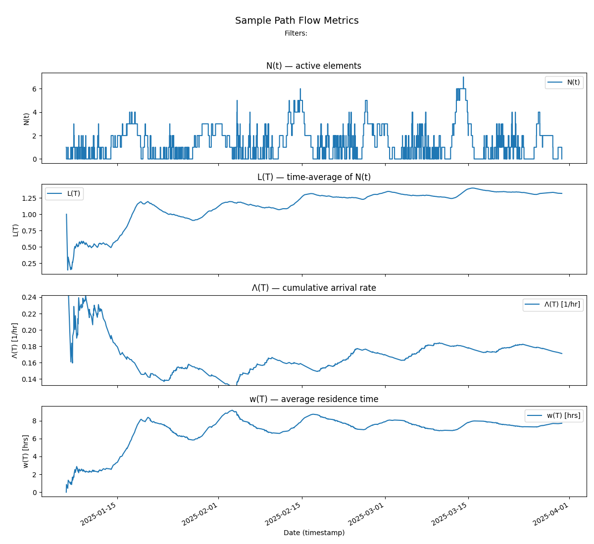
Recall that the sample path for L = λW is given by N(T) - the instantaneous number of items that are in progress at any point in the observation window.
Here is the sample path for Team Kanban
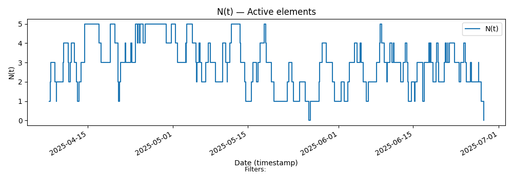
Key characteristics
Limit of 5 items in progress.
WIP rarely resets to zero
Variable size items means we can see longer stretches where items are in progress even when most items start and finish quickly.
Here is the sample path for Team XP
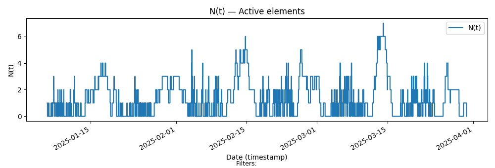
Key Characteristics:
Alternating patterns of long and short pieces of work between weeks.
WIP resets to zero at the end of each iteration.
There is no theoretical limit on the number of items in an iteration.
The time spent on any item is limited by the timebox to be at most one week.
The constraint is that every iteration delivers a meaningful increment to users (across all items).
On the surface, the two teams have very different policies and processes, and traditionally Team Kanban would the considered the team that optimizes for flow of work.
Let’s see how that plays out with data.
The Flow Metrics
Recall that sample path flow metrics measure the parameters of the finite version of Little’s Law.
This invariant is expressed as an equation involving three functions of time, derived from a finite sample path N(t) over an interval [0,T]:
Given
L(T): the time average of N(t) over [0,T]
Λ(T): the cumulative arrival rate over [0,T]
w(T): the average residence time over [0,T]
The invariant states:
for each point in the observation window, where the quantities L(T) and w(T) are derived from calculations over the cumulative area under the sample path at each T.
Please see our post “Little’s Law in a Complex Adaptive System” for formal definitions and details on how these quantities are defined.
The sample path and finite window metrics for Team Kanban are shown below. We can see Little’s Law at work in the evolution of this sample path. Overall the process is convergent since L(T), Λ(T) and w(T) all stay bounded.
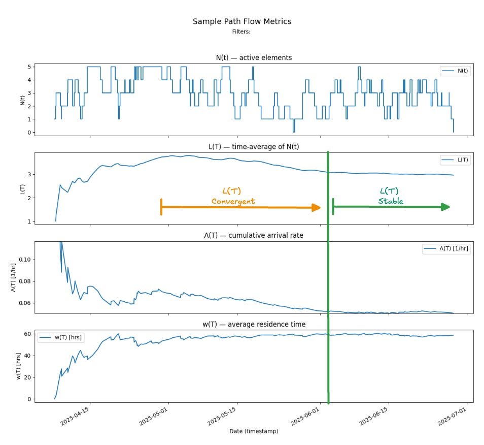
We can also make the stronger claim that the process is stable because Λ(T) and w(T) converge to a single finite value and stay there over the latter third of the observation window: as a result, L(T) also converges to a limit that is the product of the two limit values.
We see this below.
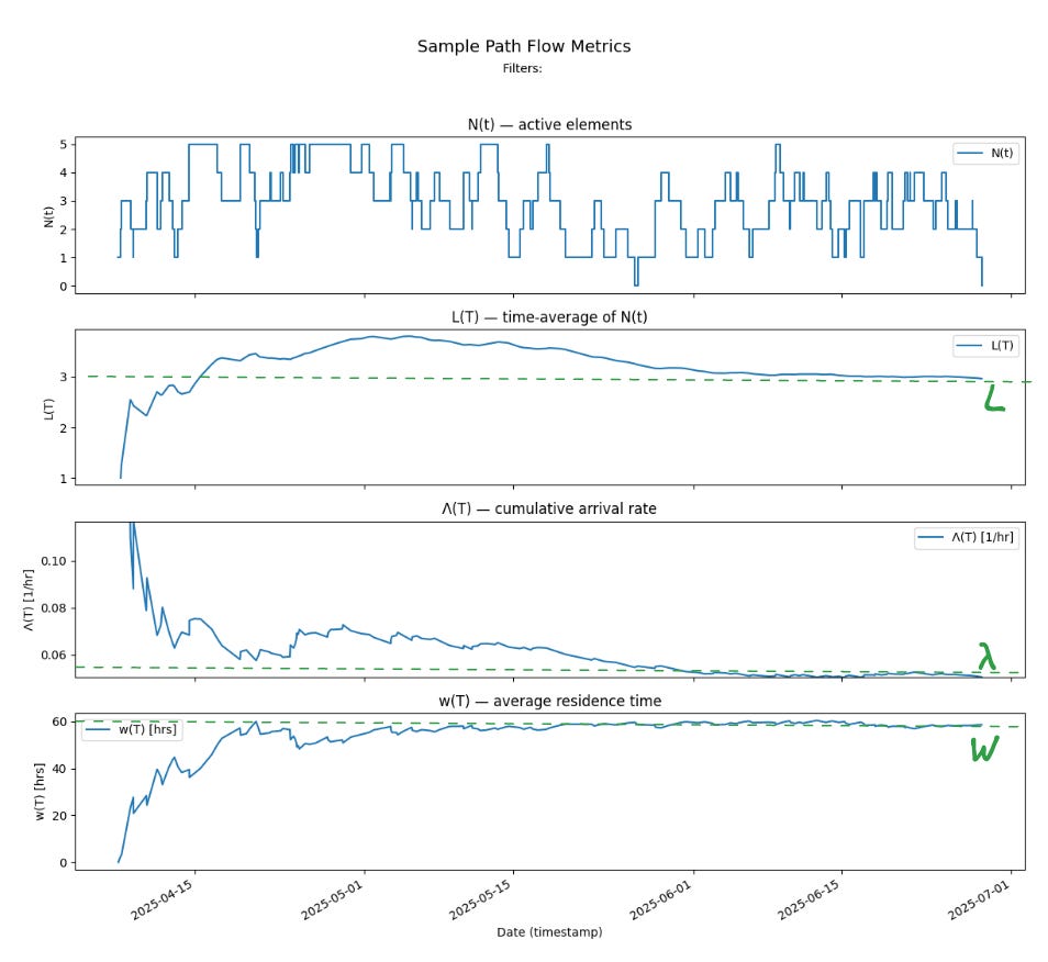
In this case:
The limit value of cumulative arrival rate λ = 0.05 items/hour or 1.2 items/day
The limit value of average residence time W = 60 hours or 2.5 days
L = 3 items is the time average if the number of items in progress
And L = λ.W, which is precisely the result that is predicted by Little’s Law.
Why does this process stabilize?
The key fact to remember about the three sample path flow metrics is that the three values are locked together by the finite version of Little’s Law at every point in time on the sample path- this is the key invariant that governs the physics of flow.
If L(T) changes it is because either Λ(T) or w(T) or both changed, and the new value of L(T) is the product of those two values.
Knowing Λ(T) and w(T) completely determines L(T)
These are deterministic causal rules: the invariant relationship between the three parameters means we can analyze “how” the process stabilizes over time using these rules embedded in the finite version of Little’s Law.
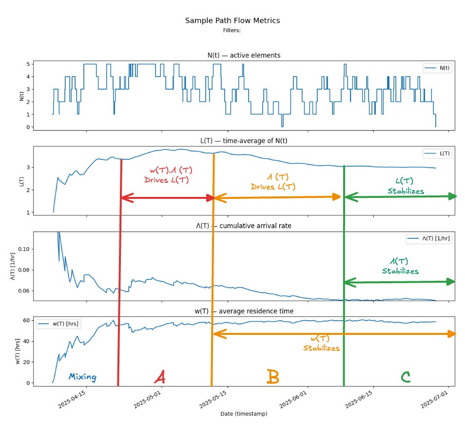
As we observe the process over a single long observation window we can see four major periods.
An initial “mixing” period of about 2 weeks where the observation window is still too small to capture the true dynamics of the process, and we are mostly measuring transient noise while averages stabilize3.
Period A - where the averages Λ(T) and w(T) have both moved into narrower ranges of values, but clear patterns of the dynamics still have not yet emerged, Here L(T) is changing as the product of Λ(T) and w(T) - so the relationships here are not linear - small changes in either parameter still lead to large changes in L(T).
Period B - where w(T) starts to stabilize. In this zone there is a nearly linear cause-effect relationship between Λ(T) and L(T).
Period C - where Λ(T) also stabilizes - and at this point L(T) also stabilizes to a product of the stable limits of Λ(T) and w(T).
Here’s why the process behaves this way.
The Kanban process constraints: the WIP limit and the response-time SLA, respectively keep Λ(T) and w(T) bounded. Mathematically, these bounds ensure4 that the each of the values independently converges to finite, stable values when averages are taken over sufficiently long observation windows.
Little’s Law then says that L(T) also converges to a limit L and that L = λ.W at the limits.
To understand what “convergence” means intuitively - consider the convergence of Λ(T):
You can see from the plot of N(t) that the arrival patterns in period A are distinctly different from those in period B. The process behavior shifts — arrivals and completions mix in new ways — but by period C, the new arrivals no longer change the overall cumulative arrival rate Λ(T) in a meaningful way.
In other words, the process has converged: we’ve observed enough of its history that adding more data (extending the observation window) no longer alters the long-run averages of the flow parameters. The empirical averages have stabilized, and the process now behaves as though it were stationary over this window.
Note that there is no guarantee that this wont change in the future - this is where processes in complex adaptive systems differ from simpler processes in repetitive manufacturing.
But this also means that shifts in these averages imply significant changes in the internal workings of the process or the external environment in which the process is operating, or both - we are seeing “new history”. Sample path flow metrics capture all these precisely.
So this is the stabilization mechanism in Kanban: WIP limits and response-time SLAs act as enabling constraints. If you can adhere to them—and let the mathematics do its work—the process is guaranteed to become stable over time.
Convergence or stability is not guaranteed purely because we have adopted WIP limits or SLAs - you have to adhere to those limits, measuring this on a case by case basis for each process at every point in its history, and figure out if your process is actually converging and/or stabilizing or shifting between behavior regimes - the concept we call meta-stability5.
The key takeaway is that Little’s Law ensures WIP limits and SLA’s that place firm upper bounds on the time to complete all work are sufficient enabling constraints to stabilize a flow process.
How long does it take?
It’s equally important to note how long it took the process to stabilize: nearly 8 weeks of observation - even though 80% items complete in 4 days or less and the rest complete in 2 weeks or less.
This is a normal pattern. When we are working in a complex adaptive system with high variability in sojourn times, meaningful patterns of process behavior only become apparent over longer observation windows relative to sojourn times in the process. Over shorter timescales, we see a lot of transient noise in the system vs the true flow characteristics of the process6.
In general, the time to stabilize in a process is directly related to amount of variability in the residence time and the arrival rate. The lower the variability in each parameter, the faster the averages converge to a stable value - we see all the relevant history in a shorter period of time.
In our example, the residence time converged faster than the arrival rate, but in general it could also happen the other way around as well.
Here the fact that we have a two-tiered SLA: a soft limit of 4 days on 80% of items and the hard limit of 2 weeks on all items - are necessary both to bound variability and ensure convergence. We can play around with these limits in any given context to see what is achievable given capacity constraints etc, but it is the combination of hard and soft limits on the response time constraints that drives how fast the process as a whole converges.
Sample path flow metrics reveal the true “Voice of the Process.”
The particulars of any given flow process will vary and small changes to the WIP limits, the SLA, the ability of the teams to meet the SLA etc. might have drastic impacts on how the process stabilizes, how long it takes to stabilize, and even whether it stabilizes.
Reporting Flow Metrics
Sample-path analysis is a powerful tool for systems analysts and process engineers who want to understand and improve how a system behaves. But what use are these numbers to day-to-day management of processes? Isn’t this all just theoretical?
This is the core tension when relying on technical quantities like cumulative arrival rate or average residence time. It’s not at all unreasonable to ask:
Will customers care about these metrics?
Who cares if some mathematical averages converge over the long run?
This is where Little’s Law earns its keep once again.
Even though sample path metrics seem highly technical and non-intuitive, we can also claim something practical: if a process is stable, these same metrics are exactly the right operational metrics to report.
Under stable conditions, the internal process metrics converge to the business-facing operational metrics —throughput, cycle time, WIP etc.
These long-run metrics have several advantages over the industry-standard flow metrics used today. They are stable, interpretable, and slow to fluctuate from day to day. When they do change, it usually reflects a genuine shift in the underlying process dynamics. That makes them far more useful for decision-making and for reasoning about system behavior, and more importantly for communicating with external stakeholders when things change7.
Short-window flow metrics still have their place: they provide tactical visibility into ongoing work. But they are volatile and offer little insight into the deeper dynamics driving the process. The two perspectives complement each other—short window metrics help you manage flow in the present, while sample-path metrics help you reliably communicate about what a process does free of measurement bias8.
The concepts of equlilbrium and coherence and their associated metrics provide the operational bridge between these technical metrics and business facing ones.
Equilibrium and Coherence
Sample path analysis says that when sample path flow metrics converge to stable limit then λ is also the long run arrival rate of the process, and this always equals the departure rate, λ is also a stable measure of process throughput. Similarly W, the limit of the average residence time is also the limit of the average sojourn time, which is the customer facing average response time for the process. The process is in equilibrium when measured over these long observation windows.
To complete the analysis let’s look at our sample path metrics and verify that they converge to the relevant business facing metrics when the process is stable.
Arrival Rate converges to Throughput
The upper chart in Fig 6 is the standard cumulative flow diagram for the flow process. It shows that purely viewed from the standpoint of point in time arrivals and departures the process looks stable9 through most of the sample path. The difference between these point in time arrivals and departures is precisely what we call the sample path.
But our definition of stability is much stronger: it requires the long run arrival rate to converge to a finite value, and this is not apparent simply by looking at the CFD. We have to compute the sample path flow metrics for this10.
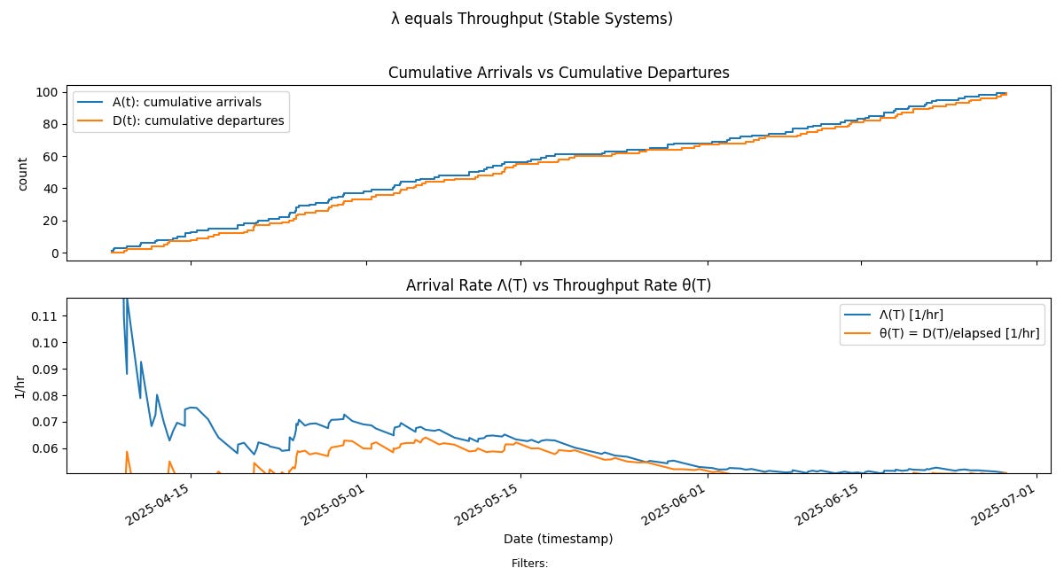
The bottom chart shows the convergence plot of arrival rate from Fig 3, overlaid with long run departure rate, which is the throughput from the process. We can clearly see that as the arrival rate converges to the limit, so does the throughput, and that the limit value of arrival rate can be substituted for process throughput over these observation windows.
Residence Time converges to Sojourn Time
The top chart in Fig 7 shows the convergence of average residence time w(T) and average sojourn time W*(T). At the stable limit, these values track each other letting us say that the average residence time is also the customer facing average sojourn time.
We discussed this convergence process in detail in our post “How long does it take?” The reader is encouraged to review that post for more details on this convergence mechanism.
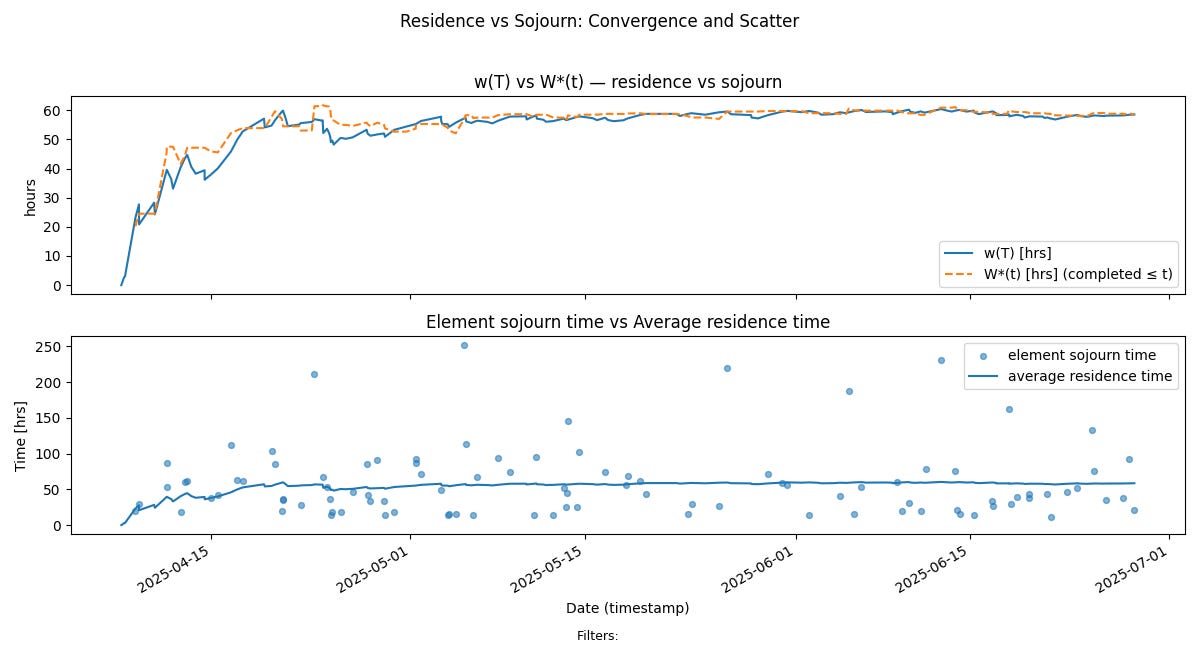
The bottom chart tracks the relationship between the average residence times and sojourn times of items.
Since residence time over long observation windows encodes both the cycle time of all items that have completed up to that point as well as the age of the in progress items up to that point, this chart captures the dynamics of both work item aging and sojourns in one view.
Since in a stable process residence time average is very close to the average sojourn time, the element sojourn times will be distributed around the residence time average, showing that internal aging remains under control across the sample path11.
Sample Path Coherence
Finally let’s put all the material above together into a simpler, easier to use top level metric that we can use to characterize flow in a process.
To recap, measuring and tracking the three sample path flow metrics:
L(T): the time average of N(t) over [0,T]
Λ(T): the cumulative arrival rate over [0,T]
w(T): the average residence time over [0,T]
give us a complete set of metrics to describe and reason about flow at all points where a process can be observed.
We’ve also see that when these values converge to finite limits, these limit values are also the same as the externally facing operational metrics of interest - sojourn time and throughput.
At any point where this happens we say that the sample path flow metrics are coherent.
In general, it is not necessary for the process to converge to a limiting value for the flow metrics to be coherent. So equilibrium and coherence are related but independent concepts.
In fact, there are many points along the sample path where the sample path flow metrics are coherent even if the process itself is not stable. In a convergent process, there are usually even more points along the way where these metrics are close enough to each other that in practice the sample path flow metrics serve as useful proxies for the externally facing metrics.
In Little’s Law in Complex Adaptive Systems we showed how to measure the empirical sojourn times W*(T) and arrival rate λ*(T) that lets us assess how often a process is coherent along its sample path by measuring how far away the product λ*(T).W*(T) from the value L(T) at each point in the observation window.
We can visualize this using a pair of scatter plots
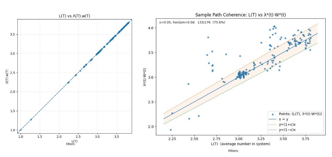
The plot on the left hand side plots t L(T) vs Λ(T).w(T) and since these are always equal per the finite version of Little’s Law, all points will lie on the x=y line. The plot on the right show L(T) vs λ*(T).W*(T) and these will points will lie on the x=y only when the process is coherent.
The right hand plot shows how often the difference L(T) - λ*(T).W*(T) remain within a fixed tolerance ε. The plot shows that for our process, Little’s Law “applies” within a 5% tolerance for 75.6% of the points on the sample path.
This sample path coherence metric is very useful global process metric to assess how far away the process is from stability over the entire sample path at any point in time.
The number shown in figure. X includes all the transients and instabilities at the beginning of the measurement, and it is helpful to suppress those by only looking at a suffix of the sample path where these numbers have started to stabilize.
For our sample path, removing the first 20 days of observations, we get the following sample path coherence chart - which indicates that the sample path flow metrics remain within 5% of externally facing business metrics for 96.1% of the sample path excluding the initial mixing period.
When comparing across processes, the first metric is the one to use, but when comparing the same process across time, it is much better to use the metric after the mixing period has been stripped out.
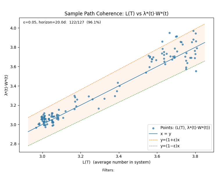
This truly shows that the combination of WIP limits and SLAs has given us a stable, coherent process!
Now we can quantify and precisely measure:
What it means for a process to be stable.
When it is safe to use sample path flow metrics for business facing decisions.
How far away a process is from being stable at any given point in time.
And do all this with nothing more than start and end timestamps - ie none of this relies on our knowing how the process behaves internally.
In the next post we will highlight this last point by using the exact same techniques to analyze the process for Team XP. We’ll see that even though that is also a very stable and coherent process, the mechanisms by which stability is achieved are quite different from the ones for Team Kanban.
What about the flow metrics we use today?
Despite being rhetorically adjacent to Little’s Law and queueing theory, our industry-standard flow metrics: cycle time, throughput, WIP, work item age, flow efficiency, and so on, that are widely used and implemented in various tools are not very effective for reasoning rigorously about flow in real-world software development processes.
These metrics provide descriptive statistics that capture process behavior at points in time or over short reporting windows. What they do not reveal are the underlying mechanics of flow. They do not model or expose the cause-and-effect relationships between what happens inside a process and how the process behaves as a result.
With the current generation of tools and techniques, our measurement practices still depend on people observing processes over short time windows, trying to interpret transient noise in the data, and drawing conclusions based on intuition rather than on the first principles that govern flow and its dynamics.
Having built measurement systems using the conventional definitions and studied reams of operational flow data from production software processes in this space for nearly a decade, I firmly believe that the techniques I’ve described here are necessary to bridge the measurement gaps in reasoning about flow in the industry.
The shortcomings in current industry practices are both conceptual and practical. They arise from how metrics are implemented in tools and how foundational ideas like Little’s Law are taught and applied by practitioners: we are not measuring the right things in the right way to reflect the true physics of flow in software development processes.
Sample path analysis is a foundational technique in building the next generation of operational measurement systems for software development.
Coming up next: Team XP
In the next post, we will do the same analysis for team XP. As a teaser, here are the sample path flow metrics for that process.
The reader is encouraged to run the analysis in Fig 3, 4 and 5 with this chart and ask the following questions:
Is this process convergent, if so why?
If so, why does it converge?
We will discuss the answers in detail and contrast with the Team Kanban flow process in part 2.
Stay tuned or subscribe if you want to get the update when it drops.
Note that we are not questioning whether these techniques are effective - they are quite effective at the small team level, but much less so when we scale beyond that. The question is why? And can we develop the theory and practical techniques needed to bridge the gap?
All data that we use here is generated via simulations.
Many of our first generation flow metrics tools only measure processes in these transient zones, and then measure each of the flow metrics as separate numbers rather than as a tightly linked trio of metrics that move together under invariant relationships.
Technically, finite bounds on Λ(T) and w(T) alone don’t guarantee convergence. Additional rate-stability conditions on N(t) and the cumulative age of work items are also required. In practice, though, if a team consistently adheres to WIP limits and SLAs, these conditions are automatically satisfied — and they can be verified directly from operational data. We will discuss this point in more detail in the next post where it will be germane to arguing that the process is stable.
We’ll see meta-stable behavior much more clearly in the Team XP process behavior, but this can also happen in the Kanban process.
Think of this as the generalization of what happens on an assembly line where everything takes roughly the same amount of time and the rate at which work is fed is constant. If the system is stable and convergent the mechanism of stabilization is the same per Little’s Law: it simply unfolds over a longer timescale.
It goes without saying that like all flow metrics, sample path flow metrics are backward looking averages. They don’t say anything about how the process will behave in the future. All the usual caveats apply when using them to forecast future behavior, and especially in planning. However a stable/slowly changing average built on long run observations is the first step in constructing meaningful statistical distributions and probability models for the process, so the sample path analysis can be viewed as the first stage of building such models etc for a flow process.
The Presence Calculus is largely concerned with analyzing the relationship between long run stable flow metrics and their counterparts over the short run. This is still a very different approach from what current flow measurement systems do. We will have more to say about this in future posts, but if you want to read ahead, much of the technical machinery is described in “The Presence Calculus: A Gentle Introduction.”
In the informal sense that we use it in the field today - this is largely an artifact of the WIP limit, not true stability in the sense of being able to apply Little’s Law.
This also shows why CFDs are not a reliable tool for assessing process stability in a complex adaptive system. The CFD only captures the input to the stability analysis using Little’s Law. It’s helpful to quickly diagnose spikes, but this information is already explicitly encoded in the sample path. The real stability analysis happens over the area under the sample path.
The scatter plot is the familiar “cycle time scatter plot” if you have used tools like Actionable Agile. By overlaying it with average residence time we can quickly check the impact of internal aging on the sojourn times.