
The Many Faces of Little's Law
Its not just for managing assembly lines

If you’ve worked in software delivery or followed any Lean or flow-based methodology, you’ve almost certainly seen this formula:
This is a formula that shows that there is an underlying “physics” to the flow of work in software, and that these key flow metrics are not simply isolated descriptive statistics.
The relationship between Throughput, WIP and Cycle Time show up in books and flow metrics dashboards, and the formula is almost always referenced in training materials to justify WIP limits, to reason about delivery times, to explain why queues form. It is part of the Lean software development canon.
The formula is usually introduced without much further qualification, as “Little’s Law.” This is directionally correct, but it’s not the full picture.
What we’ll call the throughput formula came to lean software from its applications in manufacturing. In that domain there are set of assumptions that can be made, that allow us to treat this formula as something that holds generally, in that context.
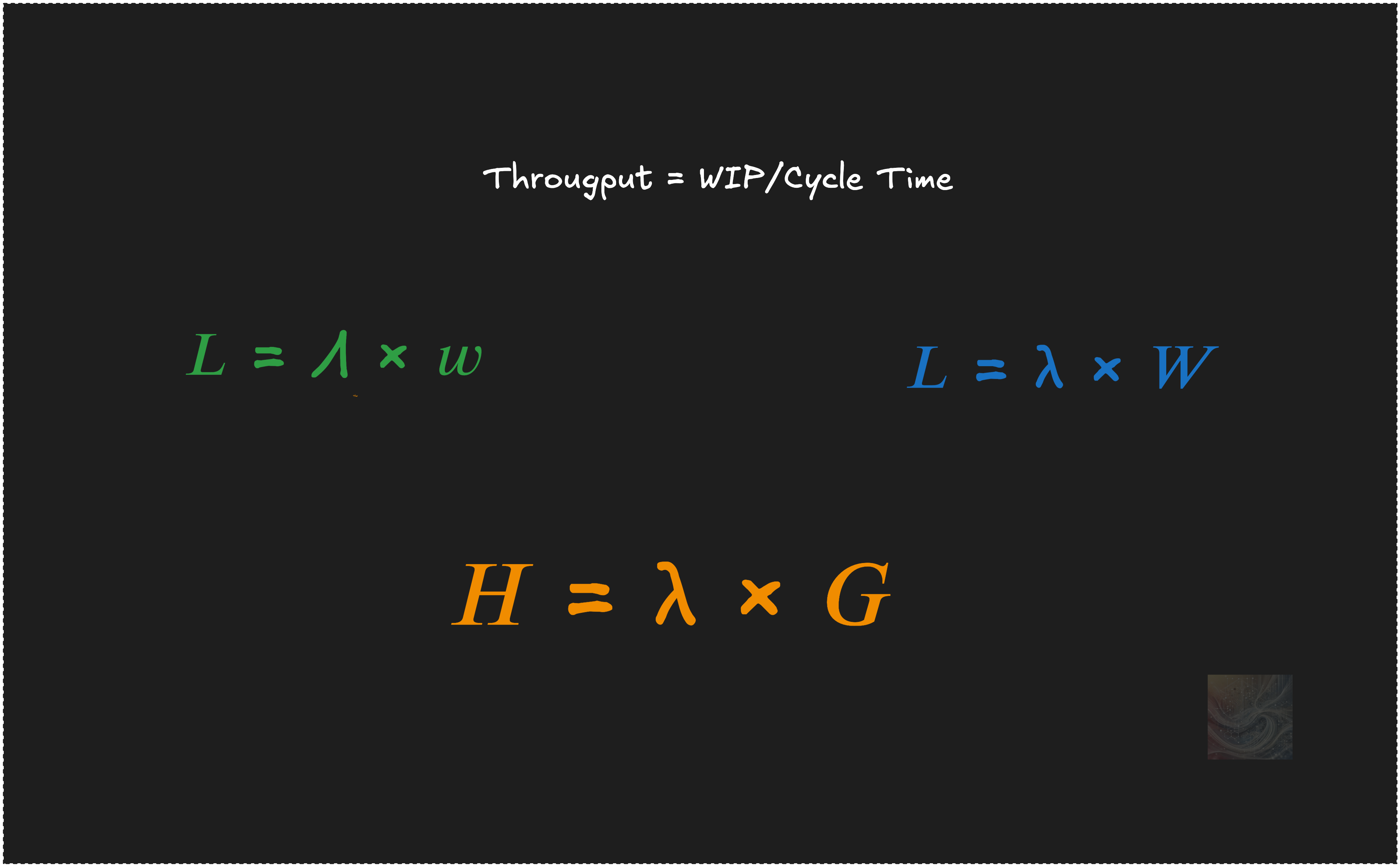
It is also well known that this formula is a rearrangement of a more fundamental identity:
This identity relates the long-run average number of items in the system (L), the average arrival rate (λ), and the average time each item spends in the system (W).
Under steady-state conditions, when arrivals and completions are balanced and the averages converge to finite values, you can simply replace λ with Throughput, and interpret L as WIP and W as Cycle Time and the throughput formula emerges.
But those steady state conditions often don’t hold—especially when measuring software development processes.
Observation windows are short, often shorter than the time span of work. Work starts, stops and arrives in batches. Work items may span reporting cycles. Under these conditions, if you just plug in the numbers for Throughput, WIP and Cycle Time from your flow metrics dashboards into the throughput formula, you’ll find that the equation fails to hold.
This is sometimes taken as evidence that Little’s Law “doesn’t apply to software,”
But this is demonstrably false. It reflects a fundamental misunderstanding of what Little’s Law is now understood to be.
If you’ve ever had folks give all sorts of esoteric or emotional arguments for why Little’s Law is irrelevant in software, this post will argue that perhaps it’s worth understanding the full power of Little’s Law before making that argument.
So let’s dig into what “Little’s Law” really says.
The Principle behind Little’s Law
There are many ways to state “Little’s Law”. But all versions follow from a single universal principle:
The total time accumulated in an input-output system by a set of discrete items, when averaged per item, is proportional to the time average of the number of items present in the system. The proportionality factor is the rate at which the items arrive at the system.
This is a conservation principle relating time averages and sample averages of time accumulation in an input–output system. It is general and universal.
More importantly, it is provable mathematically. We can clearly characterize how and when the principle holds. Unlike many “laws” that circulate in software and operations, this one leads to physical laws whose validity we can test directly knowing that it must hold.
Given the time average of the number of items, the arrival rate, and the average time each item accumulates in the system, the principle says these quantities are linked: if we know any two, the third is completely determined.
Knowing that Little’s Law holds reduces the number of degrees of freedom for change in the system. It gives us a strong model for reasoning about proximate causality in any context involving these three variables.
If I know that L changed, the only possibilities are that λ changed, or W changed or both. The product of their new values will always equal the new L. Any other explanation must ultimately be traced back to a change in one of these two other quantities.
Note that this does not let you predict how the values will change in the future, but it constrains how it can change.
Recognizing that this general principle exists makes it simpler to model and apply Little’s Law in contexts very different from the manufacturing setting implied by the throughput formula.
And this is the key - understanding that there are many different versions of a the law that we can derive contextually from the same underlying universal principle.
As 50+ years of research in academia and industry have shown, the list is larger than you might imagine and has many significant applications in software development as well.
The Finite Version of Little’s Law
The core conservation principle applies even if the system is in flux—so long as all measurements are taken over the same time window. In this sense, the most general version of the law is the one that applies to a fixed, finite time window:
The fact that the we use upper case Λ and lower case w is not a typo. These are not the same quantities as in the familiar steady state version of the law, but closely related to them.
If we look at a finite observation window T where the window is shorter than the time accumulated by items, we will see many different configurations in which items overlap that window: some start and end within the window, others start before and end inside, and still others span the entire window.
But if we focus on the observation window itself, we can consider the way in which items accumulate time strictly within the window.
This leads to a set of observer‑relative quantities that on their own obey the conservation principle relative to that observation window.
Λ is the cumulative arrival rate over the window - like the arrival rate, but includes everything that was already present at the start of the window as an “arrival”. You can think of it as over-estimate of the true arrival rate.
w is the average time accumulated by the items within the observation window - this is conventionally called the residence time of items in the window. You can think of this as the underestimate of the true time in the system.
L is the time-average number of items observed over the window. This is the exact value of the time-average of the number of items.
Little’s Law for finite windows states that the identity 𝐿 = Λ × w always holds for any finite observation window. It holds at all times and at all timescales and it does not matter whether the system is at equilibrium or not.
In this sense, it is truly a physical law. Mathematically, it is a tautology.
But crucially, even though the two quantities in the right hand side are estimates in the finite version, the estimation errors cancel out over any finite window of time, yielding the true value of the time-average of the number of items in the system!
This is a remarkably powerful universal constraint governing time accumulation in any input-output system.
The problem of end-effects
So what’s the catch? Well - clearly the difference is that λ and W in the well known version of Little’s Law represent measures on the complete items and not partial ones. In classical queueing theory, λ is the long arrival rate (rather than the cumulative arrival rate) and W is the long run average sojourn time (rather than residence time).
When dealing with business processes we are ultimately interested in talking about arrival rate and sojourn time rather than cumulative arrival rate and residence time over finite operational window. If we take a customer facing view, they represent rate at which customer requests arrive in the long run, the time it takes to respond to those requests etc. So these are the numbers that are operationally significant to a business.
To understand the relationship between the two sets of measurements, we can consider zooming out and observing the system over a window that is much longer than the time accumulated by individual items in the system (sojourn times).
Over sufficiently long windows, the time and item averages measured over that finite window are dominated by the measurements on complete items rather than partials. The partials become “end-effects” that become less significant as we take measurements over larger and larger windows.
The identity L=λW holds in the long run, because as the end effects vanish, cumulative arrival rate and average residence time converge to the (true) arrival rate and average sojourn time respectively. This is the intuition behind the formal proof of what is now considered the definitive statement of Little’s Law.
Short Windows vs Long Sample Paths
Think about how data is gathered and used operationally.In software, flow metrics are almost always reported over windows - a week, two weeks, a sprint etc. that are determined by the business process being used Scrum, Kanban, SAFe etc, and not usually based on how long things actually take to move through the process.
But many meaningful “items”: features, defects, and epics often take longer than these reporting windows. That means the data in any reporting window includes partial work: some items started earlier, some are half done, some finished in a window, some won’t finish for weeks.
As a result, trying to apply the throughput formula or even L = λ × W to an operational window directly, produces inconsistent numbers. Arrival rates don’t match completions. Work appears and disappears midstream. The law “fails” not because the math is wrong, but because the quantities being plugged in are not measured over a consistent observation window. This is the real reason why Little’s Law “doesn’t hold” when you typically measure it in operational flow data.
This is also why the finite-window version, L = Λ × w, is critical. It relates measurements that are actually observable in a consistent interval. Even when the observations include partials or the system is shifting between operating modes, the relationship holds. There are many operational uses for this, but we wont go into that here - that will be a topic for future posts.
Sample Paths
Our example above suggests that if we observe it over a “long enough observation window” we will get an alternative, and perhaps more meaningful set of numbers for measuring flow.
But how we decide what is long enough?
This is where a powerful analytical technique called sample path analysis comes in. It is the foundation for the mathematical proof for L=λW and the concept can also be used quite directly in an operational setting.
The idea is that instead of measuring flow metrics over short, rolling observation windows, we observe the system from a fixed starting point in time and observe it continuously over a long enough window (weeks, months, years etc - as long as necessary). In the context of Little’s Law the sample path we observes is items in the system at any point in time - the instantaneous WIP. The observation window is the length of the sample path.
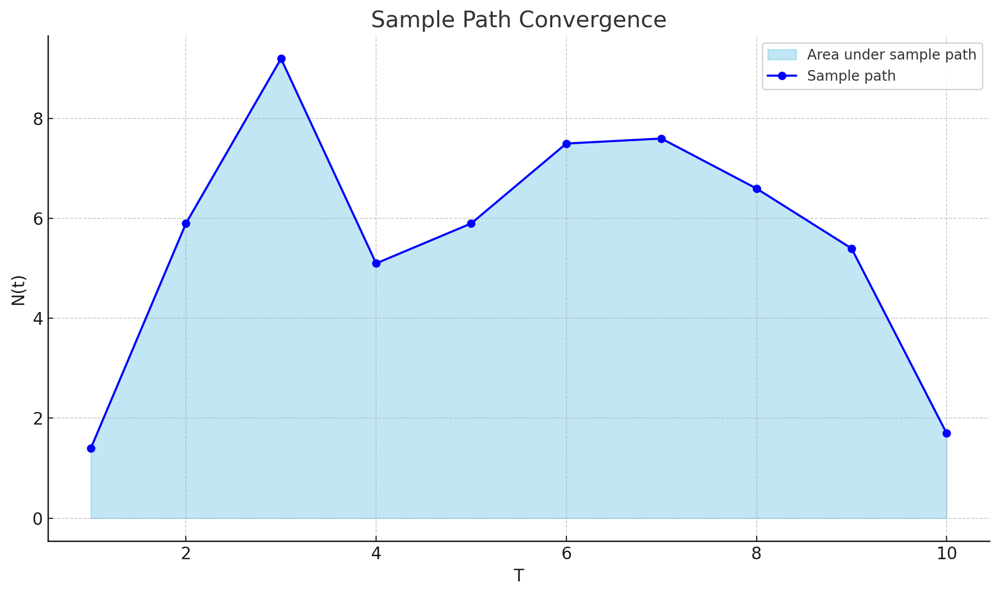
For a sample path a finite length T , if N(t) is the number of items in the system at time t, the time average of the number of items in the system over the interval T is given by the ratio of the area under the sample path to T.
Now the question becomes do the estimation errors in the finite observation windows always vanish and become negligible if we observe a sufficiently long sample path.
The answer is, not always: The classic proof of Little’s Law by Stidham shows that they vanish if L(T) converges to a finite limit over a sufficiently long T.
This leads us to the critical ideas of convergence and divergence.
Convergence and Divergence
If we observe a sufficiently long sample path we only have two possibilities to consider.
First possibility: the system settles down, after a finite window of time. Practically, this means that if we measure the quantities the finite version we’ll find that the quantities L(T), Λ(T) and w(T), in the finite version they will converge to finite limits L, Λ, w and these limits will correspond to the L, λ , and W of the steady state version of Little’s Law.
This, in fact, is the key result that was proven by Dr. Shaler Stidham in 1972 and is now considered the definitive statement of Little’s Law.
That is, if Λ → λ and w → W as T → ∞ then L = λ × W .
But what if these limits dont exist? Then work continues to accumulate indefinitely, arrivals outpace completions, residence times stretch out indefinitely—we get divergence.
This is the more useful distinction: not whether the “system is stable,” but whether or not long run averages on a sufficiently sample path converge to finite limiting values.
In practical terms Little’s Law says:
If the cumulative arrival rate Λ(T) converges to a finite limit as T grows,
and the average residence time w(T) converges to a finite limit as T grows,
then the limit L = λ × W exists and holds.
If not, the system is divergent, and divergence tells us something real: the system is structurally unbalanced. Items are backing up, time in system is growing, arrival rate is overwhelming capacity.
This shift—from seeking “steady state” to detecting convergence or divergence—is critical in domains like software, where systems are rarely in equilibrium for long.
All of these parameters can be precisely measured on operational data.
In fact, the minimal length of the sample path over which a system achieves convergence is critical characteristic of its input-output behavior. One that Little’s Law shows us how to calculate quite precisely.
Thinking about convergence and divergence gives us a much richer vocabulary for reasoning about the relationship between micro behaviors of the system over short operational windows and macro behaviors of the system over long sample paths.
Convergence vs Stability
It is important to understand that convergence, as defined above, is more general than the concept of “stability” often discussed in the context of flow metrics.
Little’s Law states that the long‑run relationship L = λ × W holds as long as the limits L, λ, and W exist. It does not require these limits to remain constant over time. In convergent systems, these values can and do change, and when they do, they are still constrained to obey Little’s Law—just as in the finite‑window form.
We will reserve the stronger condition of stability to those systems where the finite limits of the long run averages themselves stay constant over time. Many repetitive and assembly line processes satisfy this condition, but software development processes often don’t, and they don’t need to for Little’s Law to apply.
In this sense, Little’s Law applies for equally to linear and non-linear system, complex adaptive systems, deterministic and stochastic systems, and even certain types of chaotic system.
Such systems may be convergent, and Little’s Law may apply with different parameters over different periods of time. but the system is not stable or predictable in the sense that we normally associate with stability.
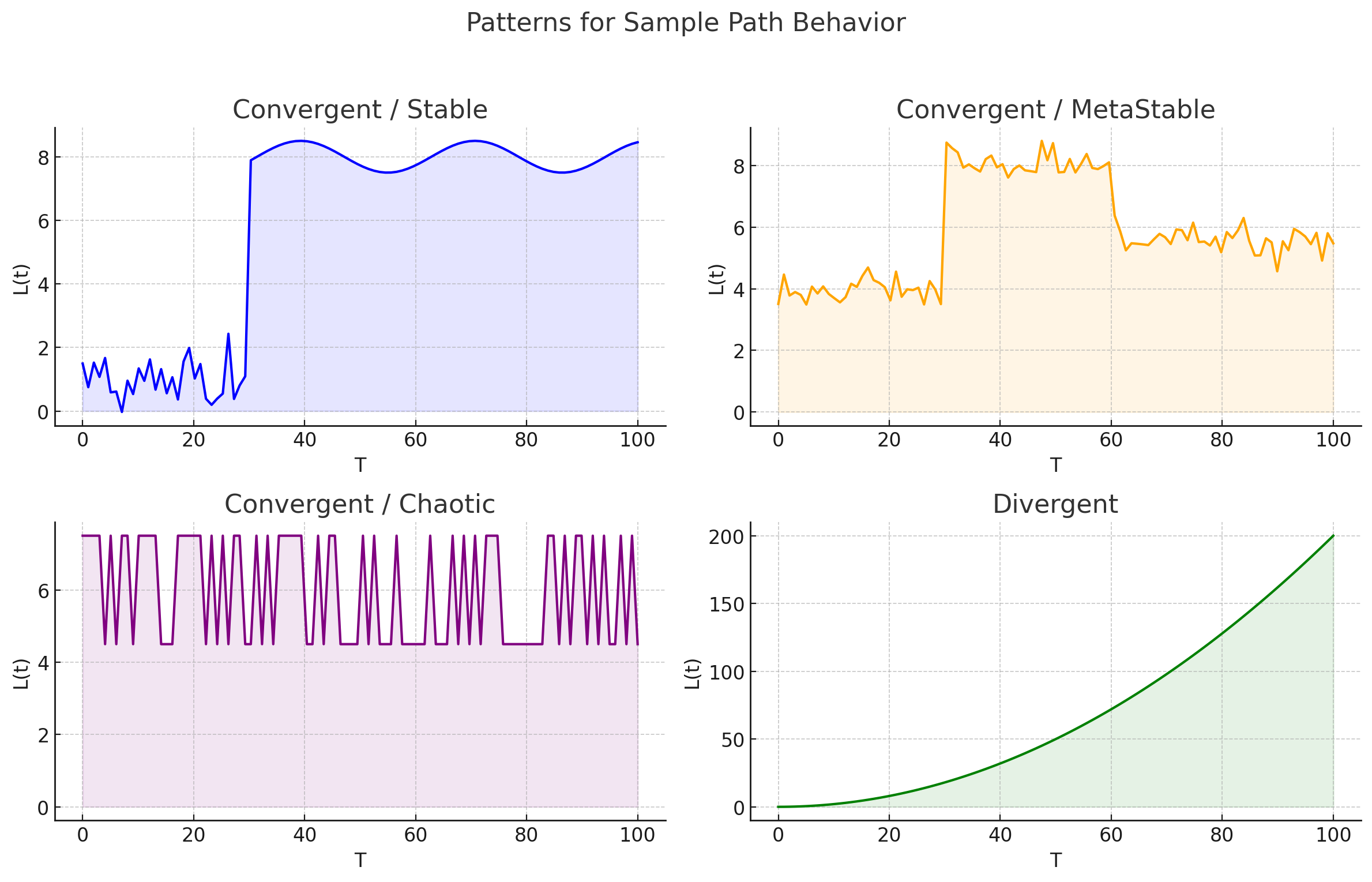
Fig 4 shows some of the possibilities here (there are many more). Certain processes like CI/CD pipeline can be strictly stable like in the first example. The second example of meta-stability, where the system remains convergent, but the limits in Little’s Law shift over time is characteristic of most processes that involve humans and machines. Truly chaotic processes are rare in the SDLC, but not impossible. Every one of these behaviors is convergent.
And all these process can tip over into divergence if the system is structurally unbalanced (they can also usually be brought back into convergence). The power of the law is that it does not care about what kind of system it is internally. And every one of the different types of systems described above can exhibit both convergent and divergent behaviors depending upon the structural balance that the existence of the limits implies.
But we can use still reason about these systems with Little’s Law, both over any finite window of time, or over long sample paths, using the appropriate definition of the averages.
So far from being a tool that lets us look at simple, linear or deterministic systems, Little’s Law in its more general form is one of the most powerful general purpose analysis tools available to us for analyzing input-output system regardless of their internal structure or behavior.
This type of reliable “black-box” analysis of systems can provide very valuable first pass insights into how a system behaves, without having to know any of the internal details about the system or having to know what kind of system we are dealing with.
Equilibrium and Coherence
There is another, very useful way to think of the difference between observing an input-output system over short fixed observation windows vs observing it over a long, continuous sample path.
We can think of the fixed finite version as a point in time snapshot of an typical operator’s view of the system. In general, for real-time reasoning, it is reasonable to assume that we make decisions not over complete histories, but only the parts we can observe. We will need to estimate parts of the system history that it cannot observe. The fixed window version captures this very well.
The steady state version reflects what the items (or customers) themselves experience from the system over the long run - but their “experience windows” may not always align with the operators observation window.
“Equilibrium” can then be considered as a state where the operators view aligns with the customer’s view. It is a state of epistemic coherence across different observers in the system, where they each make their own measurements and end up agreeing on their values (within some error tolerance).
Both perspectives are hugely important, but the advantage of the finite version is that we can reason about the operators view locally using the finite version of Little’s Law from moment to moment with only partial information, and also get a sense of how far away from “equilibrium” the system is over a given finite observation window. The finite version is usually much more volatile. The equilibrium view provides a slower changing perspective of the macro behavior of the system.
Operationally, having both views in perspective is a big deal in software development, because we are typically operating far from equilibrium. Most operational tools that measure flow metrics don’t make this distinction, and there is a lot than can be improved on this front.
There is much more ground to cover on operationalizing all this. The references at the end of this post are a good starting point, and we will have more to say about this in future posts.
But let’s continue our exploration of Little’s Law by examining an even more general version - this is an economic interpretation of the law, and it is considered the most general form of Little’s Law.
𝐻 = λ × 𝐺: the economic version of Little’s Law
What is truly remarkable about Little’s Law and something that is rarely exploited is that the same conservation principles holds even when we’re not tracking time accumulated by items, but some other time varying quantity: costs, risks, revenues, profits etc that can be tied back to the items.
In this framing, suppose each item contributes some “value” to the system expressed as some at a time-varying function: call it fₖ(t), for item k. So instead of a set of items, we have a set of time varying functions of items.
Lets look at a single instant of time. Summing all contributions across the functions gives H(t), the total value accumulation rate in the system at time t. Similarly looking across all the items and computing the cumulative value of each function over time gives us G_k the total value contribution from item k.
Similar to L = λW can define:
H = long-run average value of the accumulation rate H(t)
G = average value contribution per item 𝐺 across functions = ∑𝐺ₖ ⁄𝑛
λ = arrival rate of items
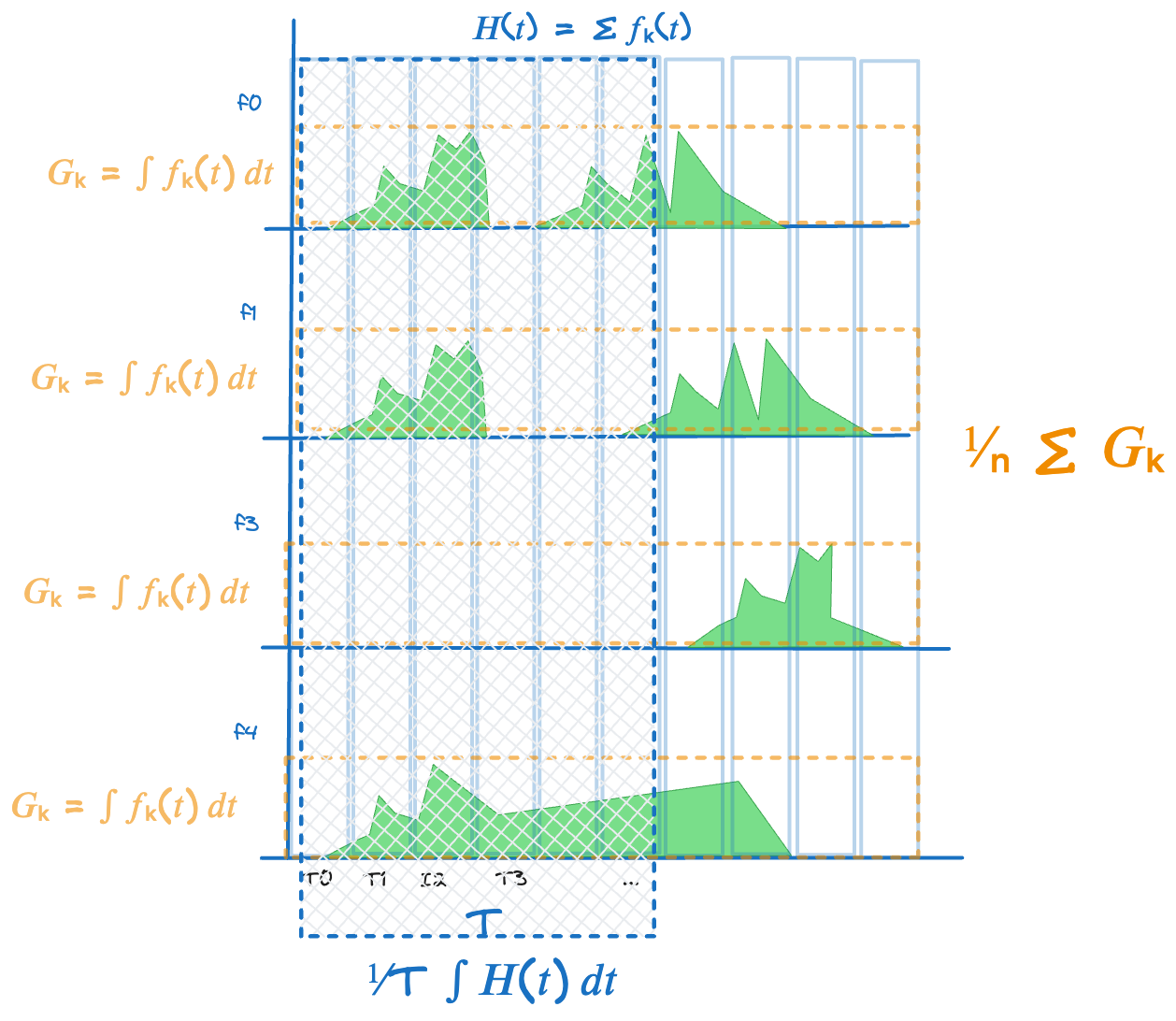
Then using the same approach of measuring these parameters along a sufficiently long sample path we can derive both finite and steady state version of Little’s Law the leads to the most general form of Little’s Law that states that if the long run values λ and G converge to finite limits, so does H and then
This general form opens up a much wider set of modeling possibilities. We can use it to model the time varying interaction of complex functions of items - for example how risk accumulates, how customer satisfaction scores rise, or how delay-related cost builds over time—all without relying on any specific process model for the underlying behavior: just observed input output behavior.
In short this is a mathematically rigorous, and operationally tractable way of modeling the physics of the “flow of value” and not just the flow of “work”.
When modeling the flow of value in value networks, this formalism and Little’s Law in this general form will prove to be a valuable analytical tool.
But there are many, many more useful ways in which this general form of Little’s Law can be exploited and we need much more machinery in place to make this easier to use and apply in practice settings.
We discuss this in the section on further reading at the end of the document.
Why Little’s Law matters
When applied correctly, Little’s Law gives us something rare: a strict constraint across quantities we can observe. If two change, the third must follow. It doesn’t tell us what will happen. It tells us what can’t happen. It works as a check on our measurements, as a signal for divergence, and as a very sensitive set of levers by which we can actively steer systems that operate far from equilibrium.
But for that to work, we need to stop treating Little’s Law as a formula that only applies to stable factories, and realize that treating it as a conservation law allows is to use it meaningfully for general input-output system including nonlinear and complex adaptive systems that are never in equilibrium for long.
For software teams, this means:
Use the finite-window form (L = Λ × w) for real-time analysis across normal operational windows.
Use the classical form (L = λ × W) once you’ve validated convergence using sample path analysis - report these as the system level flow metrics and use these to target system improvements.
Think in terms of identifying sources of divergence and feedback mechanisms to move divergent systems into convergence.
Use time-value generalizations (H = λ × G) to measure and manage accumulations of costs, risks, benefits and rewards that can be modeled as time-dependent functions of items.
There is a whole other parallel set of “flow systems” with mathematically precise semantics that we can build on top of our familiar flow system built on the flow of discrete work items.
Little’s Law is the foundation for building such models.
Further Reading
In this post we made a lot of general claims without too much by way of detailed explanations or proofs to back them up. What we have described above is a summary of nearly 50 years of research and development in both academia and industry in the field of operations research.
Much of this research, its history and its significance seem to be unrecognized in the software industry and this post was intended to provide a broad strokes introduction.
While Little’s Law started out as a simple empirical observation about waiting lines in operational settings, it has led to deep and lasting mathematical results that revealed that it is a much more fundamental law than the simple throughput formula we are all familiar with.
Of course, all this needs more than hand-waving to make real in an operational setting. If you are interested in understanding the underlying theories and arguments in more detail and how to start applying these ideas in practice here are a few follow up resources.
The best reference source for understanding the theory and history of the law is the survey paper, “Little’s Law on its 50th anniversary,” that Dr. Little wrote on the 50th anniversary of his original proof of the law.
For a much more detailed version of the current post, and one that builds upon this survey paper and introduces the ideas here in a form that is more meaningful to folks in the software development community - see my post “A Deep Dive into Little’s Law”. This has a detailed list of references that I feel are directly relevant for applications in our domain.
“Sample-path analysis of queueing systems” by El-Taha and Stidham is the definitive reference to the mathematics underlying all these ideas and much more. This is mathematically dense read and is not meant for practitioners. Its useful if you want to learn and understand why the results we will leverage in applications are true.
But if you are less concerned with theory and want to start applying these ideas directly, all this material is the foundation of The Presence Calculus, a reframing of the underlying techniques used in proving Little’s Law in all its forms, into a modeling and measurement substrate that is easier to apply and use in practice and also for us to build operational tooling around. I expect to be writing much more extensively on this topic in coming weeks, but a fairly comprehensive overview of the presence calculus can be found in our introductory document The Presence Calculus: A Gentle Introduction.
The Presence Calculus Project website has all the material that we will be publishing on this topic - including papers on the formal theory behind the calculus as well as the practical application use cases.
The Presence Calculus Toolkit is an open source library that we are building to operationalize the concepts in the presence calculus. It is not yet ready for production use, but we plan on using this as a reference implementation for the measurement and modeling primitives of the presence calculus.
Post script: For those of your familiar with the Little’s Law through Wikipedia and or queueing theory texts, you might be surprised that we have introduced Little’s Law without referring to queueing theory, stochastic processes, or probabilistic assumptions like ergodicity and stationarity, that are typically understood as being required for Little’s Law to hold, and as originally proven by Dr. Little.
In fact, Dr. Stidham’s proof of L = λ × W showed that all these were superfluous conditions and that the law was a completely deterministic result that could be applied to both deterministic and stochastic systems without knowing what kind of system it was.
We cover these proofs and their history in more detail in our deep dive into the history and proofs of Little’s Law.
Dr. Stidham’s sample path analysis technique, which yields a proof of Little’s Law as only one possible application, is a much more fundamental and powerful tool and we operationalize in the presence calculus.