
What is Residence Time?
Its not a cycle time by another name

In “How long does it take?” the previous post in my series on Little’s Law, I focus on the importance of a metric called residence time. It’s a fundamental concept you need to know about in order to understand how Little’s Law and flow metrics really work under the hood.
Also, it has huge value as a day-to-day operational metric in it’s own right.
But the concept is probably unfamiliar to most people — even those well-versed in the principles of flow and flow metrics. Recently, a number of people have asked me if residence time is just another name for concepts they already know: cycle time, lead time, flow time, and so on.
Yet another common question has been whether this term refers to the time a process a spends in a specific work flow state like development or QA - this is also called cycle time or flow time in various parts of our community1.
It isn’t.
Residence time is a fundamentally different concept, and it is worth understanding what it is. In this post, I’ll explain the relationship between residence time and the flow metrics we already know very well.
The standard flow metrics
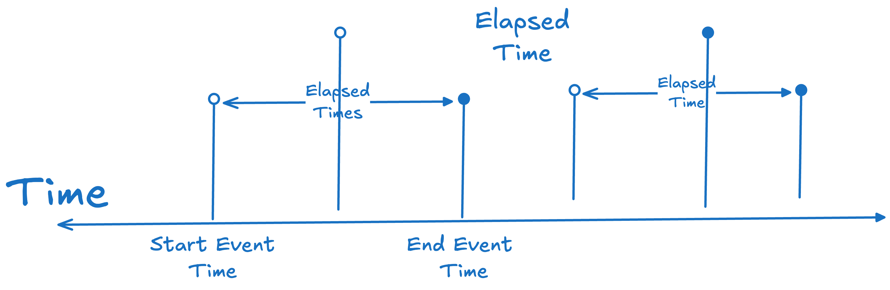
Let’s look at the familiar metrics we use today—lead time, cycle time, flow time etc. All are elapsed-time metrics. Each measures the time between two events that mark the beginning and end of some process in a system:
Project approval → delivery to customers
Customer request → fulfillment
Feature is available for acceptance testing → Feature is accepted
Defect is logged → fix deployed to production
PR is opened → PR is merged
Practitioners use different name like lead time, flow time, cycle time etc for these metrics, and also the same terms with different meanings: there is a fair amount of inconsistency in the way we use these terms today in the industry.
But whether we call it a lead time, cycle time or flow time, the important thing is not the specific name: it’s the definition of the start and end events and their domain semantics.
Also, what matters is that they are measuring different underlying processes. For a given process it is useful to have a generic term that refers to the time it takes to complete that process from start to finish - we will use the term sojourn time for this.
Sojourn time
In classical queueing theory, a queue serves as an abstraction for such processes2. The events are arrivals and departures at a queue, and the elapsed time between arrival and departure is generically called sojourn time.
“Sojourn” is a neutral term: it simply means time for an item to “travel across” the queue, or to be processed. All the elapsed time metrics we see in practice are all just different flavors of sojourn time. So we’ll adopt sojourn time as our generic term for such metrics. In this sense, lead time, cycle time, flow time as defined by various practitioners are all sojourn times for some underlying process.
The average sojourn time for a process is an important operational metric because is the W in Little’s Law3:
But residence time is not a sojourn time. It’s a completely different concept.
Here’s why we need it.
Average sojourn time is tricky to measure when variability is high
Sojourn time is always item-relative. You measure the elapsed time for a given item from start event to end event.
You can compute an average of sojourn times of a set of items easily if you have a set of start and end events for those items. But this implies you can observe the whole journey of all the items and know when they start and finish.
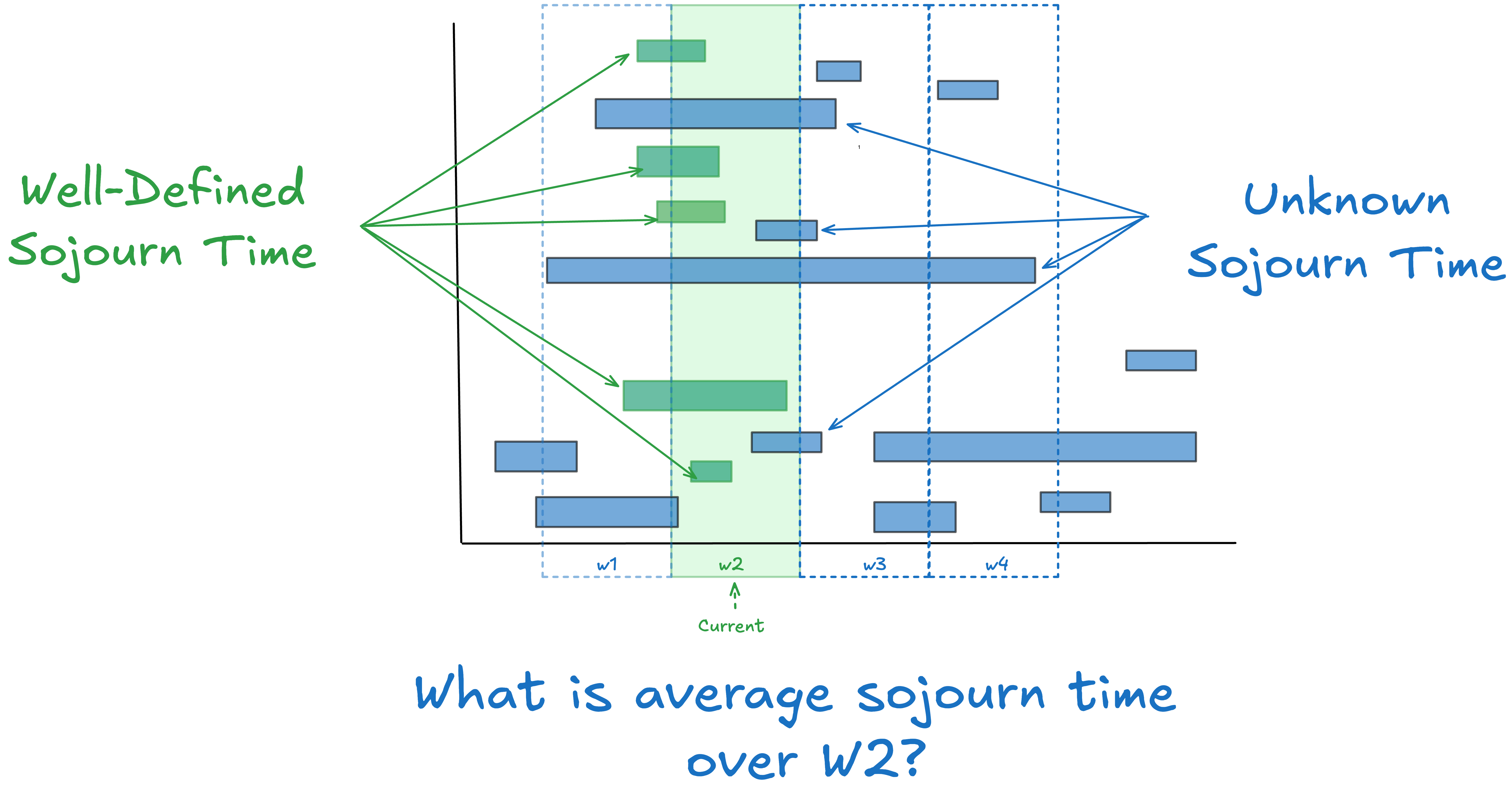
In reality, we often observe processes mid-stream. Some items are already in progress when we start observing, or haven’t yet finished by the time we stop. Their start or end times might be unknown. Other items start or finish during the window. Other start and finish during the window.
This matters because when we measure the three quantities L, λ and W in Little’s Law they have to be measured over the same observation window before you can even consider applying any of the machinery of the law.
What kind of average sojourn do you get if you can’t observe the whole journey and are simply observing the process over some arbitrary finite window of time?
The standard approach is to measure average sojourn time for the items that end in the observation window. Pretty much all the standard definitions of lead time, cycle time, flow time etc in use today assume this. In Fig 2 these would the average of the green bars, but these averages are not being measured across W2 - you need to expand the observation window to capture all the events involved.
We discussed the problems this creates in our post last week
How long does it take?

This is the first in a series of posts exploring specific applications of sample path analysis in complex adaptive systems. We introduced this topic in broad strokes in Little’s Law in Complex Adaptive Systems.
The problems raised here are not theoretical problems. The reason that the three flow metrics as we measure them today don’t obey Little’s Law is because they are not being measured across a consistent observation window4.
Enter residence time
Residence time is a new kind of elapsed time metric that can be applied to any finite observation window. Residence time is not item-relative but observer-window-relative. If I observe a process over the window [0,T] residence time measures the portion of each item’s elapsed time that overlaps with that window.
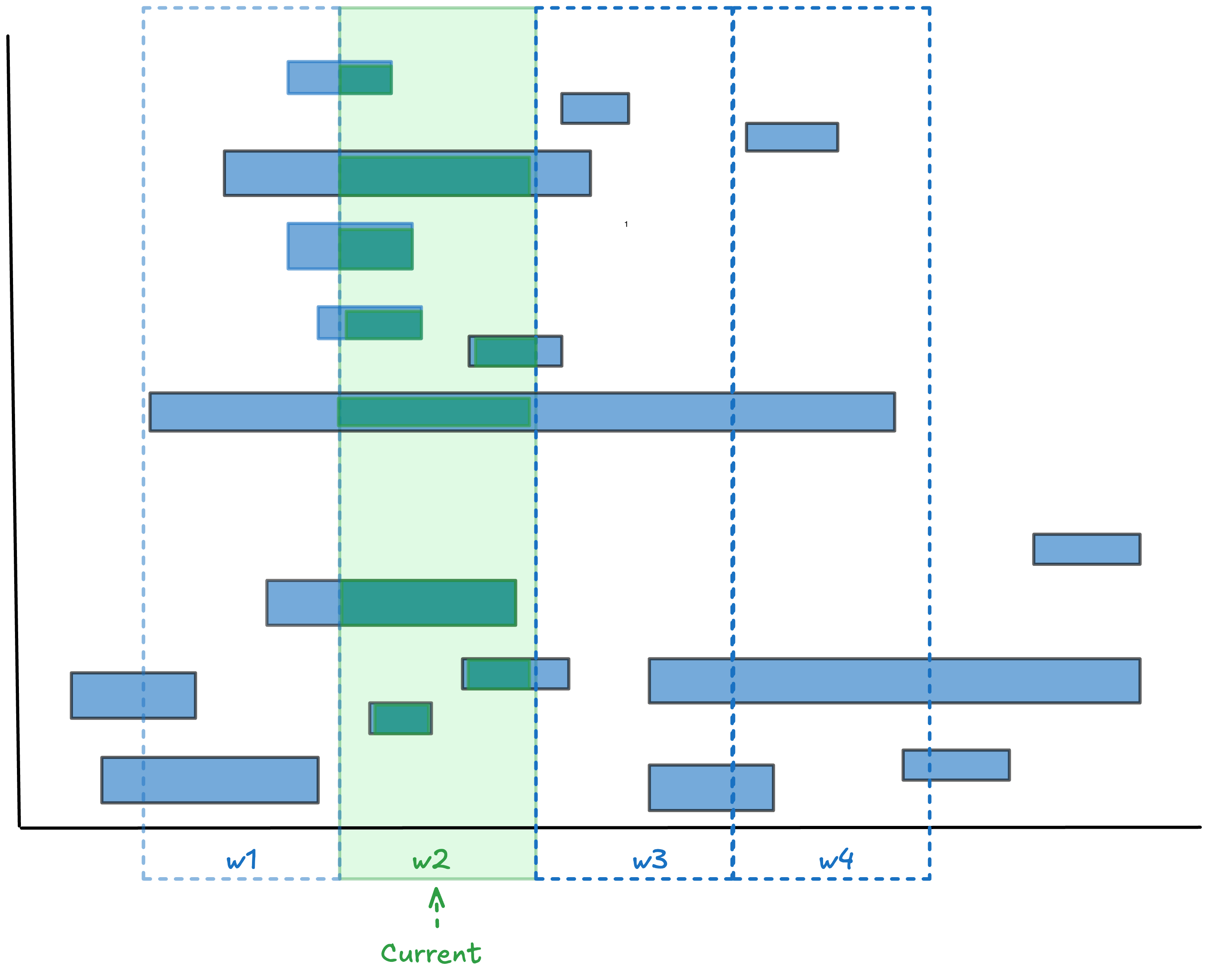
In Fig 3 these are the durations shown in green. Because residence time is “clipped” by the observation window, it’s always less than or equal to the full sojourn time for any given item5.
We can define two different kinds of elapsed time averages for given a set of items.
Their average sojourn time across some set of items (over some large unknown horizon) that includes all their start and end points: W,
Their average residence time in a finite observation window [0,T] as w(T).
Now we have two averages which are both well-defined but are potentially defined over different observation windows.
Given any sojourn time, we can define a related observation-window relative residence time.
Now the question becomes are there any observation windows where you get the same average value when you measure both quantities simultaneously6.
Residence time is a key measurement in sample path proofs of Little’s Law, so measuring processes using residence time mirrors how those mathematical proofs show how and when Little’s Law holds.
The relationship between residence time and sojourn time.
As we discussed in The Many Faces of Little’s Law, average residence time, w(T) plugs directly into Little’s Law at any finite observation window.
This holds unconditionally, for any observation window, as long as L(T), Λ(T), and w(T) are also measured over the same window. This means that residence time is always well defined over any finite window, and we can also define a corresponding well-defined version of arrival rate and number in the system such that the finite version of the law holds for any finite observation window.
This is one big difference between residence time and sojourn time - the identity in Little’s Law holds for sojourn times only under equilibrium conditions.
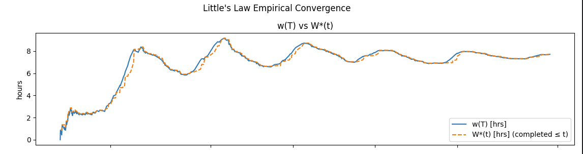
The relationship between sojourn times at equilibrium and residence times becomes clear when we measure them over long observation windows: windows much longer than the sojourns themselves, as in Figure 4.
Little’s Law says that if w(T) converges to a finite limit over sufficiently long observation window T, then that limit value W is also the average sojourn time of the items over those sufficiently long windows.
In these long windows, total residence time of items in the window can be decomposed into two parts: the sum of the completed items’ sojourn times plus the accumulated ages of the incomplete items.
This is the key property of residence time. Over short window, it looks like we are adding up bits and pieces of time. Over long observation windows, those bits and pieces become sojourn time and work item age, and it unifies the time accumulated by completed items and items in progress into a single number.
As the window grows, if the unknown future sojourns of incomplete items become negligible relative to the total sojourn time of completed items, then the average residence time and average sojourn time converge toward the same value. But this convergence is not guaranteed. Whether or not it happens provides a powerful way to distinguish two fundamental modes of process behavior: convergence versus divergence.
If a process is convergent, the average residence time w(T) approaches a finite limit as T grows. Over that window, average sojourn time W also converges to the same limit. ie in a convergent process, the average residence time equals the average sojourn time over a sufficient large observation window. That’s when we can replace w(T) with W in the Little’s Law formula say Little’s Law “applies.” to the process.

Fig 5: Convergent metastable process If the two values converge to a single value and stay there forever, then the process is stationary and we can simply use that limit value as the average sojourn time W in Little’s Law. This is also a good stable value to provide as your operating characteristic for process time and monitor it for changes.
But more likely, you’ll get processes that behave like the one in Fig 5. These are convergent but the values of w(T) and W(T) come together and drift apart as the process evolves, but as long as they stay within a tolerance of each other, we can use residence time as a very accurate proxy for sojourn time.
This kind of process is called metastable, and in a complex system this is what we should expect residence times and sojourn times to look like most of the time.
If a process is divergent, the averages never converge no matter how long you observe the process. So you can never apply L= λW to that process. And measuring residence time and sojourn time together, makes this divergence visible early.
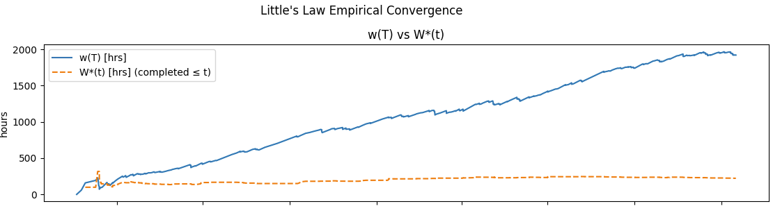
This is why residence time is by far, the operationally more useful metric. Sojourn time is useful to report metrics after the fact, but residence time is what lets you really understand the process dynamics from moment to moment.
Operator vs participant view
There is another way to look at the relationship between sojourn time and residence time.
Sojourn time is the participant’s view—how long the customer experienced in the process.
Residence time is the operator’s view—how much of that elapsed time was visible within an operational window.
When these two align on average, we say the flow metrics are coherent.
The bottom line
Residence time is more than another name for cycle time. It’s a complementary, but necessary lens to measure any given elapsed time metric reliably when processes sojourn times are much larger than the standard measurement window and/or the processes move continuously in and out equilibrium - as most software development processes do.
Sojourn time tells you how long an item spent from start to finish. Residence time tells you how long that item was “present” in your observation window whenever you observe it over any period of time.
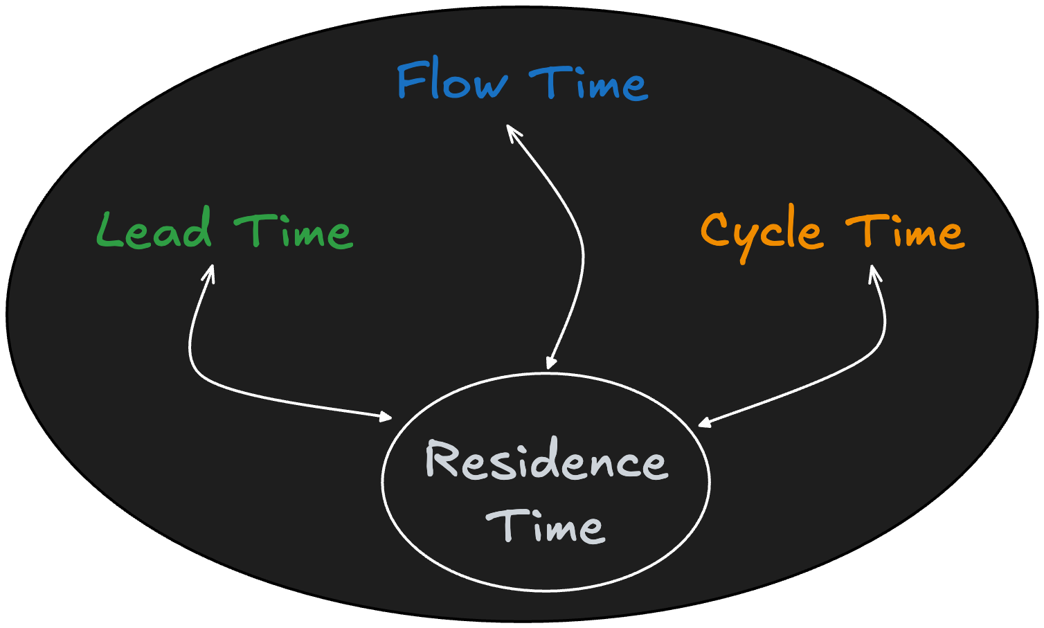
So a good way to think about it is as shown in Fig 7:
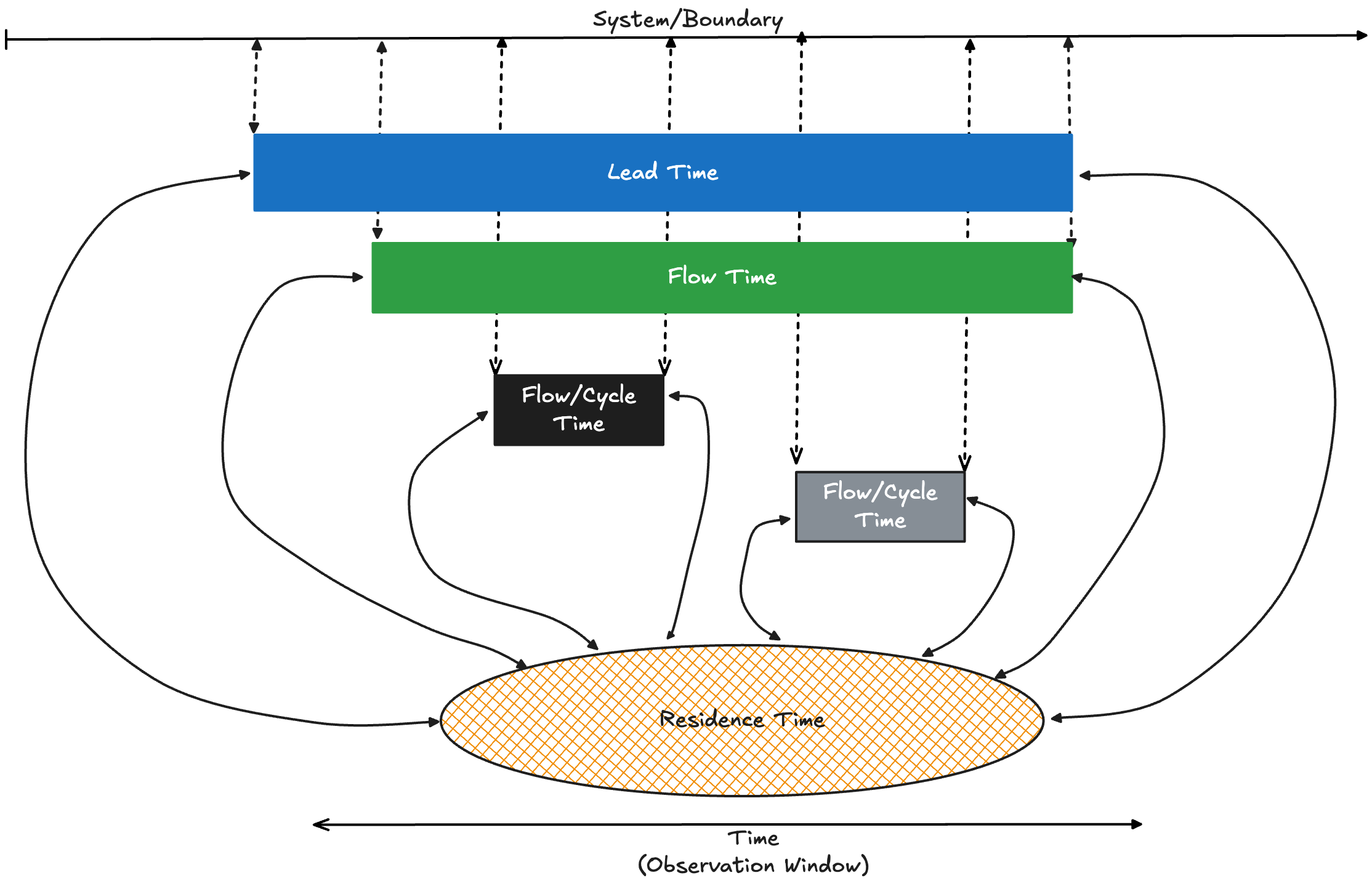
For any sojourn time metric you can define for a flow process, there is a corresponding residence time metric. The relationship between average residence time and average sojourn time over sufficiently large observation window let us determine how close or how far away the process is from a equilibrium state per Little’s Law.
This applies to lead times, cycle times, flow times etc - any sojourn time metric you can define.
It is also important to remember that convergence/divergence is not a system property but a process property. In applying sample path analysis, we think of lead time, cycle time etc as representing different processes at different granularities (potentially nested within each other).
Each of these processes may be convergent or divergent independently, and it is possible that the they impact each other’s convergence/divergence. Sample path analysis will not all explain these interactions but will show the impact of those interactions via convergence/divergence of each process as measured over a common observation window.
Thus the first step to understanding the dynamics of these processes is to understand whether each of them converges or diverges.
Then we can start asking why they behave the way they do.
We discussed how this type of causal reasoning might work in
The Causal Arrow in Little's Law

Most people think Little’s Law is about stability. But what it says about causality is even more important.Thanks for reading The Polaris Flow Dispatch! Subscribe for free to receive new posts and support my work.
The Causal Arrow in Little’s Law.
Check that post out for more on how we can use these metrics to reason about systems.
Let me know in the comments if this is still confusing or whether I can help make this clearer.
The term residence time is used in performance analysis of computer systems to refer to the time an item spends in a particular queue in a network model of a computer system. Some operations books also use this to define the time spent at a specific service station. In that sense it could be said that we are inventing a new meaning for this term here. But we have two counter-arguments.
First, the term residence time is not commonly used in any of these senses in the software development flow community - we use cycle time or flow time for this, and this is already confusing as it is.
Second the most important sense in which residence time is used in those other operations management contexts is that they assume that one can unconditionally apply Littles Law to a single node/station using residence time. This assumption does not hold for flow time or cycle time in software, but the definition of residence time as the observation-window relative elapsed time preserves this semantics.
So the key thing about residence time that differentiates it from all the other operational elapsed time metrics is the fact that we can always plug it into the finite version of Little’s Law and in combination with the cumulative arrival rate, apply Little’s Law to reason about flow at all points in time.
In particular, processes where we want to understand the ratio of time spent waiting to time spent processing - queuing theory is the study of waiting in processes.
Dr. Little himself called W “waiting time” in his writing, but queuing theorists needed to distinguish between time “waiting for service” and “in service”, so they reserved sojourn time for W and queue time for “waiting for service”. So this confusion around naming these things goes back decades - not a new phenomenon. Bottom line is define start and end events that demarcate initial and terminal conditions for your process and call the time between these sojourn times generically. You can rename them whatever you prefer in your context, provided you do it consistently in your context.
The standard measurement of average WIP also suffers from similar problems - but in general the problem of verifying whether Little’s Law applies is entirely a problem of figuring out how to construct a consistent measurement window over which we can measure all three parameters of Little’s Law in a well-defined manner.
Although average residence time for a finite window can be greater than the average sojourn time for the items that finished in that window. This may seem paradoxical but it it’s really not. Whenever we look at an item that has not completed, its residence time is less than its sojourn time - but some of that sojourn time lives in the future. In any finite observation window, the residence times of incomplete items may be much bigger than the sojourn times of the completed items in that window. So the averages residence time in a window can (and often is) larger than the average sojourn time for that window.
The non-obvious part here is that the averages may match even if not all the items being measured in both sets match up perfectly, but as long as they are being measured over the same observation window, the discrepancies become irrelevant over sufficiently long windows - this is what Little’s Law allows us to claim.
Another great entry in the series, thank you.
I found Figure 7 confusing.
If I understand correctly... Lead Times describe, let's call it a Lead Process, and Lead Process has *a* Residence Time measurement. Flow Times describe a Flow Process, and Flow Process has *a* Residence Time measurement, which is notably different from Residence Time measurement of the Lead Process. Cycle Times describe a Cycle Process, and Cycle Process has yet another Residence Time measurement different from the others.
Fig 7 makes it look like they are all the same Residence Time. Which, they're not. They share the name, but they share "Residence Time" like Lead, Flow, and Cycle share "Time". To me, Fig 3 style communicates best, and Fig 7 strikes me as counter to everything I read up to now.