
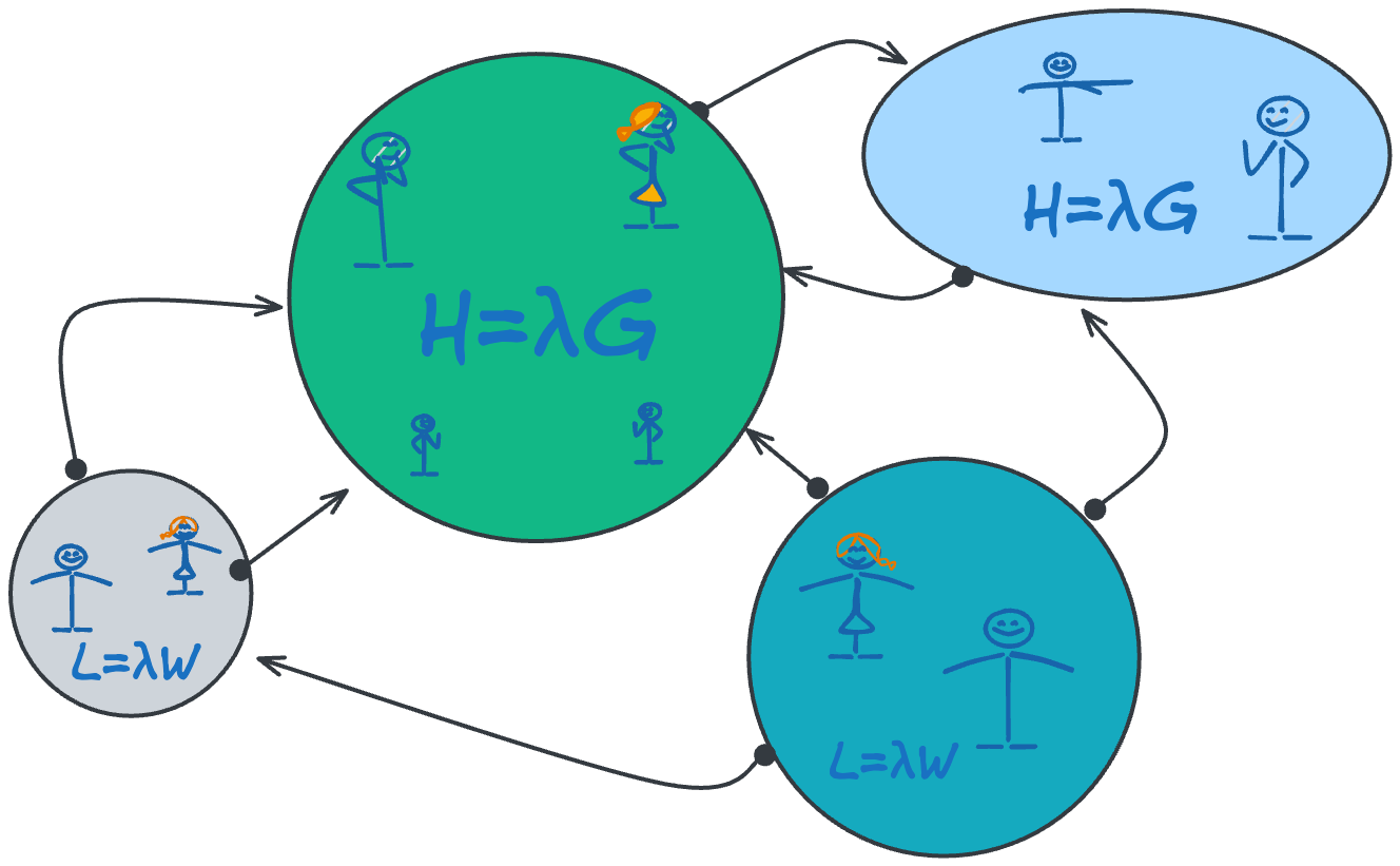
Little's Law in a Complex Adaptive System
Applying sample path analysis to real-world software product development

Introduction
A central thread in our series on Little’s Law is this: when Dr. John Little first proved Little’s Law, he did so using the mathematical machinery of stationary stochastic processes. Rooted in probabilistic arguments, his proof showed that the relationship L=λW held for stochastic processes under two strong assumptions: that the underlying probability distributions were strictly stationary (not just the mean, but every statistical moment, variance, skew, and so on, remains invariant under time shifts) and that the arrival process was ergodic1.
Those are very restrictive conditions, but they are only sufficient conditions. If they were necessary, the law’s domain of application would be quite narrow—limited mostly to highly automated, low variance machine-centric environments like industrial production. Even there, strict stationarity rarely holds. Once humans enter the loop, the assumptions collapse very quickly.
Process-control techniques—pull policies, WIP limits, and the like—are often deployed both in industrial production environments and lean software development: to approximate stationarity and create localized approximations of stability. But under Dr. Little’s strict framing, even these approximations would not suffice for the law to hold.
Industrial production processes may succeed in forcing quasi-stationarity. But with humans involved at every level, most software product development processes are inherently non-stationary. At the team level, and especially across teams, customer domains, and market boundaries, there are too many exogeneous and adaptive influences to expect stationarity or even well defined probability distributions to govern their behavior.
The question is does Little’s Law apply in such domains? The answer is an unqualified yes. We’ll make the case in this post.
We showed in The Causal Arrow in Little’s Law that if Little’s Law can be applied in a domain, this fact enables powerful analyses of process dynamics from rough-cut estimation to rigorous cause-effect reasoning. We saw in The Many Faces of Little’s Law that this opens up ways to reason about time-value and the economics of processes. So there are real-world benefits to establishing the validity of Little’s Law in given domain.
Fortunately, as we saw in A Brief History of Little’s Law, the power of the law does not hinge on the strong assumptions in Dr. Little’s original proof. In 1972, Dr. Shaler Stidham’s deterministic sample-path proof showed that the validity of the law does not need stationarity or ergodicity, or even that the underlying process has a knowable probability distribution. This opens the door to applying Little’s Law in many more domains and in complex adaptive systems in particular.
The key insight is that we can use a purely deterministic approach to analyze processes through direct observation and reason about long run behavior of sample paths. Rather than speaking about the stationarity or ergodicity of theoretical distributions, we can analyze behavior in terms of convergence and divergence of empirically observed averages which satisfy provable mathematical invariants. For operations management, this is far more practical and directly actionable.
This post digs into the technical details of sample path analysis in some detail.
We’ll flesh out the high level concepts we outlined in the The Many Faces of Little’s Law 2.
While doing so, we’ll work through a concrete case study, showing how to apply Little’s Law to a product development process for a team seeking product-market-fit. Using production data, we’ll show how to measure parameters in Little’s Law using sample path techniques, interpret what they mean in the context they are derived from, and show what meaningful inferences we can make with them.
We’ll provide rigorous but accessible explanations of the underlying mathematics so that you can see how the law works and why it holds and build an intuition of how to apply Little’s Law beyond plugging in numbers into a formula.
We hope to put to rest once and for all the widespread misconception that this is a law that only applies to simple, linear, or ordered systems, or that real-world complex adaptive systems are not amenable to rigorous mathematical or causal analysis.
About this post
This is a long post even by the standards of the Polaris Flow Dispatch. The ideas here are not too difficult to follow, but they do require some patience to read through carefully and understand the subtleties involved.
To quote Dr. Shaler Stidham from his original sample path proof of Little’s Law:
...there are many who feel that 𝐿 = λ𝑊 is such an 𝑜𝑏𝑣𝑖𝑜𝑢𝑠 relation that a rigorous proof is superfluous: at most a heuristic argument is required...𝘏𝘦𝘶𝘳𝘪𝘴𝘵𝘪𝘤 𝘢𝘳𝘨𝘶𝘮𝘦𝘯𝘵𝘴 𝘤𝘢𝘯 𝘣𝘦 𝘥𝘦𝘤𝘦𝘱𝘵𝘪𝘷𝘦. 𝘐𝘯 𝘢𝘯𝘺 𝘤𝘢𝘴𝘦, 𝘵𝘩𝘦𝘺 𝘢𝘳𝘦 𝘯𝘰𝘵 𝘱𝘢𝘳𝘵𝘪𝘤𝘶𝘭𝘢𝘳𝘭𝘺 𝘪𝘯𝘴𝘵𝘳𝘶𝘤𝘵𝘪𝘷𝘦 𝘸𝘩𝘦𝘯 𝘵𝘩𝘦𝘺 𝘢𝘴𝘤𝘳𝘪𝘣𝘦 𝘵𝘩𝘦 𝘷𝘢𝘭𝘪𝘥𝘪𝘵𝘺 𝘰𝘧 𝘵𝘩𝘦 𝘳𝘦𝘴𝘶𝘭𝘵 𝘵𝘰 𝘱𝘳𝘰𝘱𝘦𝘳𝘵𝘪𝘦𝘴 𝘵𝘩𝘢𝘵 𝘵𝘶𝘳𝘯 𝘰𝘶𝘵, 𝘶𝘱𝘰𝘯 𝘳𝘪𝘨𝘰𝘳𝘰𝘶𝘴 𝘦𝘹𝘢𝘮𝘪𝘯𝘢𝘵𝘪𝘰𝘯, 𝘵𝘰 𝘣𝘦 𝘴𝘶𝘱𝘦𝘳𝘧𝘭𝘶𝘰𝘶𝘴, 𝘸𝘩𝘪𝘭𝘦 𝘧𝘢𝘪𝘭𝘪𝘯𝘨 𝘵𝘰 𝘥𝘰𝘤𝘶𝘮𝘦𝘯𝘵 𝘵𝘩𝘦 𝘪𝘯𝘧𝘭𝘶𝘦𝘯𝘤𝘦 𝘰𝘧 𝘱𝘳𝘰𝘱𝘦𝘳𝘵𝘪𝘦𝘴 𝘵𝘩𝘢𝘵 𝘵𝘶𝘳𝘯 𝘰𝘶𝘵 𝘵𝘰 𝘣𝘦 𝘦𝘴𝘴𝘦𝘯𝘵𝘪𝘢𝘭.
I wanted this post to be a comprehensive starting point for all the essential ideas of sample path analysis in one place. In coming weeks I plan to write shorter posts that focus on specific topics in this post in greater detail and with a wider range of examples.
This material is based upon the treatment of Little’s Law in the textbook Sample Path Analysis of Queueing Systems by El-Taha and Stidham. It is the definitive mathematical treatise on sample path analysis, co-authored by one of the originators of the technique. It contains the detailed mathematical definitions and proofs of the results we use here. The treatment there is terse and my goal here is to make the mathematics more accessible to practitioners without losing rigor. Any errors in translation that appear in the post are mine and mine alone. If you find any, please let me know and I will be happy to correct if necessary.
This article may be cut off in some email clients. Read the full article uninterrupted online.
The Polaris Case Study
We’ll begin with a case study to motivate why I first got interested in this topic.
It is a story about the development of a new SaaS product. I know the story well because, Polaris, the software platform from which this publication originally took its name, was incubated to support my advisory practice. I wrote much of its technical measurement infrastructure and the initial version had powered my advisory business for several years before the period we examine in the case study.
The data we’ll examine comes from a period when we were building a SaaS version of Polaris: one that could reduce onboarding times for data collection and customer modeling, and provide configurable versions of analytics workflows and dashboards I had found useful with clients over the years.
In working with clients my practice leaned on industry-standard paradigms—flow metrics, code review metrics, work allocation breakdowns, DORA metrics etc—the same ones found in most other commercial engineering management platforms. We had our own proprietary takes on how we used these and they were reflected in the our advisory program, but they were refinements rather than a broad re-thinking of the core premises prevalent in the industry.
However, I found that Polaris was not all that effective at measuring our own product development process, even though we were a tiny team. I’ll explain why in a moment, but I found I had to go back to the drawing board and rethink core ideas behind the relationship between the flow of work and the flow of value to understand why.
Our Story
We were in the early GTM phase: a working product, a handful of customers, and rapid iteration to focusing on product-market-fit3. We balanced reactive work for customer implementations and work needed to close and onboard new clients, with filling out missing features and ongoing platform work.
Our product team was small: three engineers (myself included, doubling as product manager, tech lead, and consultant) and two senior engineers. The tech stack was modern, the codebase maintainable and well-tested, though some early assumptions from the consulting days had become technical debt as we discovered more customer use cases. We integrated frequently, and anything merged to main was automatically tested and deployed.
The data in this case shows our core product development process. Units of work were normalized to tangible customer, product, or infrastructure goals. We tracked them through single Jira stories4 across multiple deployments and customer feedback cycles. Each “story” might involve several production deployment and feedback cycles and run from a few days to a few weeks. We deployed continuously, so at any given time, we could be pursuing many outcomes in parallel with our customers. Lead times were intrinsically variable, and variability was not a focus for optimization since much of it was in the hands of the customer. We lacked a formal success metric so were not measuring “outcomes” or “value” formally even though work cadences were aligned to customer outcomes.
We avoided a large backlog. Outside of customer-reported bugs, we only tracked work we actively intended to pursue or were in process; the rest lived in documents, notes and my head and pulled in for detailing shortly before we decided to work on it. We had an efficient software delivery process (after all we were advising our clients on how to build these) and our process was more about staying responsive to customer signals and sales cycles, which were more or less unpredictable.
In our process much of the “cycle time” was often outside our control. We had a formal stream of interruptible internal work - things we would work on when there was nothing of higher priority from the customer end to work on5. Overall, we wanted visibility into the all threads in play, internal and client-facing, even if many sat idle a lot of the time6. Our way of working was to keep as many threads of customer facing work moving towards an outcome with our limited team, rather than minimizing multi-tasking and maximizing throughput7.
This workflow was quite different from what we recommended for our clients, who tended to be larger, more mature organizations with slower software delivery processes. Polaris itself had been optimized for their context. For our own workflows, traditional flow engineering paradigms were less useful: we already had efficient software delivery pipelines, and a focused intake process, so metrics like PR cycle time and aging internal tasks gave little insight. What we needed were metrics that reflected the full value delivery cycle.
But our tool, designed for clients still working on optimizing core software delivery, wasn’t well-suited for that. Many conventionally undesirable conditions like aging or idle work were simply our way of working, artifacts of representing the entire value creation cycle in our units of work.
I realized early on that like most tools on the market, our own tool was not a great fit for the companies still working this way, but that was not the market we were chasing at the time so it wasn’t a priority for us to try and solve it.
But in retrospect, I’ve come to think that the problem we were facing is the real problem to solve if we want to tackle the concept of measuring value creation at all. If you strip away all the internal inefficiency in delivering software - the upstream decision making to prioritize what to build, and the downstream product and engineering processes - you are still left with this cycle where where you are working across the customer and market boundaries to make and validate decisions on what to build under uncertain outcomes. Decisions that are partially out of your control and can take widely varying amounts of time to converge to a measurable outcome. Time to value and value are largely uncorrelated.
In retrospect, I found the idea of Value Exchanges in a Value Network a much better model for thinking about this problem. Value networks naturally span organizational and company boundaries, and the value exchanges in the network are (potentially long running) transactions between parties who then mutually assess whether each exchange was valuable over time. Our units of work were structured as value exchanges even if we were not formally measuring value. I was convinced that how we measure the “flow of value” had to focus on modeling these exchanges at the value network layer.
Even though I didn’t have the theory or terminology (and certainly not the math) to explain it at the time, our team had stumbled upon value exchanges as our unit of work by necessity, but our traditional flow metrics were not very good at capturing how “flow” at this level worked.
Why This Matters
By the standards of Dr. Little’s original framing of stationary stochastic process, our product development process would be ruled out of scope to reason about with the machinery of Little’s Law: too messy, too variable, too non-stationary to model as a “flow process” where everything, including “value” is supposed to flow smoothly and predictably, and continuously from left to right in highly stable processes.
We would be trying to stabilize the process through divide and conquer - breaking up internal work and customer validation to separate phases, and internal units of work into smaller “right-sized” pieces so they would “flow” on shorter timescales. As a result we would get great internal “flow”, but lose focus and analytical insights on the longer timescale value exchanges where value creation actually happens.
Current approaches to flow never really address the larger problem that the flow of value in the network is discontinuous, unpredictable and often not correlated to the time and resources invested in development. Smaller teams like ours have less internal cruft slowing down the internal cycle and the “flow of value” problem emerges starkly and irreducibly at shorter timescales.
In this post show how we can model and measure the flow of value exchanges using sample path analysis, focusing on time to value, and show that the long run process dynamics still satisfies Little’s Law in spite of highly variable, non-stationary behavior8.
Time to value and value are not often correlated in new product development, but typically we incur opportunity costs proportional to the former so it is still an important operational metric, and sample path analysis gives us a good way to measure this robustly.
The fact that we are dealing with a complex adaptive system does not change the applicability of these techniques. In fact they thrive under the conditions, because complex adaptive systems are inherently open and non-stationary and sample path analysis works out of the box in these types of domains.
The core techniques we demonstrate in this case study show not only that Little’s Law can be fruitfully applied at any timescale, but that it can be applied regardless of the internal structure of the processes and organizations involved.
This approach to modeling and measuring value creation cycles is now a core pillar and focus area for my practice, under active development and refinement9.
Sample Path Analysis - A Worked Example
Sample path analysis requires very little by way of data.
The minimal input is a data set with start dates and end dates (either or both of which may be unknown). Each data point represents some identifiable element from the domain under analysis. These elements need not be tangible objects in the real world: as long as each has an identifier for context, we can apply the analysis. What matters are the timestamps attached to these elements.
In the Polaris data set, an element represents a product goal or outcome whose success or failure can be assessed somehow. This could be a customer requested enhancement, a product feature an experiment or an internal technical enhancement.
The start date denotes the decision to pursue an outcome, and the end date marks the decision that the outcome was either achieved or deemed no longer worth pursuing.
Conceptually, this means we do not have to think of elements as discrete items arriving and departing from a “system.”
A complex collaborative process like product development, for example, may be treated as a black box whose behavior we can observe: a sequence of timestamps with some metadata describing what was pursued, how much time things took, what measurable outcomes they created etc. In theory, these can be sourced from transaction logs in operational environments provided the necessary book-keeping exists.
We are not concerned with how the underlying process produces that behavior or what its internal structure may be: sample path analysis allows us to make useful, general claims about the black box. More importantly, we can measure and reason about this long run behavior rigorously from just this minimal description, and with no additional information.
Flow Processes
Mathematically, the general category of input structures to the analysis are called marked point processes (MPPs) which are simply a sequence of timestamps with some attached marks (metadata). We will assume that element identifiers are available as marks.
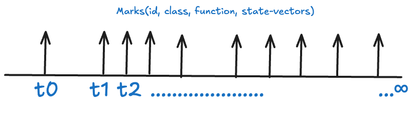
In a sample path analysis, we start with an appropriate MPP to analyze. If necessary, we do some pre-processing on raw domain data from operational logs to extract and transform the needed timestamps and metadata to construct the MPP.
Little’s Law and its generalizations apply to MPPs where the marks themselves are functions of time, ie element behaviors and their effects have temporal extent. We will call these flow processes. We analyze the accumulation of those effects over shared intervals of time.10.
The characteristic feature of flow processes is that each point event has a measurable effect that persists in time after that event. That effect can described as a function of time.
To make this less abstract, consider the following figure. Domain elements create time-varying effects within an observation window.
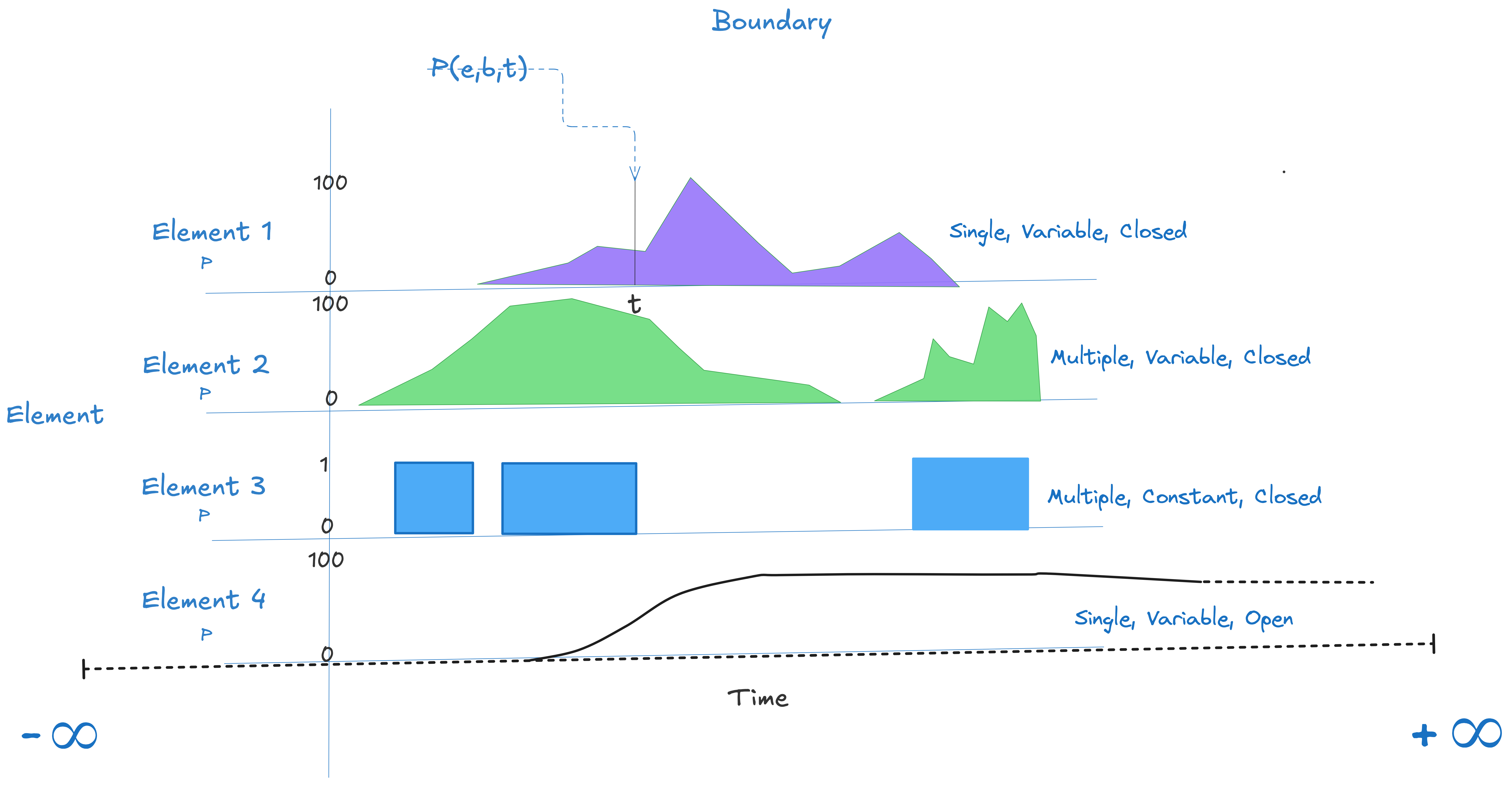
Using Little’s Law and its generalizations, we analyze the cumulative impact of the superposition of the effects over time.
The classical form, L=λW, concerns elements whose effects are recorded as simple binary presence/absence (e.g. Element 3 in figure 2) in the environment. The marks are boxcar functions which have unit values over a finite interval and are zero elsewhere. In a queueing system the timestamps denote arrivals and departures of items from the queue. L=λW is useful for answering questions like “how many” and “how long” and surfacing the precise relationship between the two.
The generalized form, H=λG allows marks that are arbitrary functions of time, not just binary indicators. In the MPP representation, these presence density functions are simply additional marks attached to timestamps. These are used to model the time-value (not time-to-value) of the elements. We will use these to quantify costs, risks and rewards associated with the elements, and connect it back to the “how many” and “how long” questions we can simultaneously ask with L=λW.
In this post we will focus on L=λW and build the foundations to talk about the more abstract concept of the flow of value via H=λG. From the standpoint of analytical mechanics, the two versions will not be very different: in all respects L=λW is just a special case of H=λG, but L=λW is significant on its own for operations management, and it is easier to build the intuition for how and why these laws work by looking at the special case.
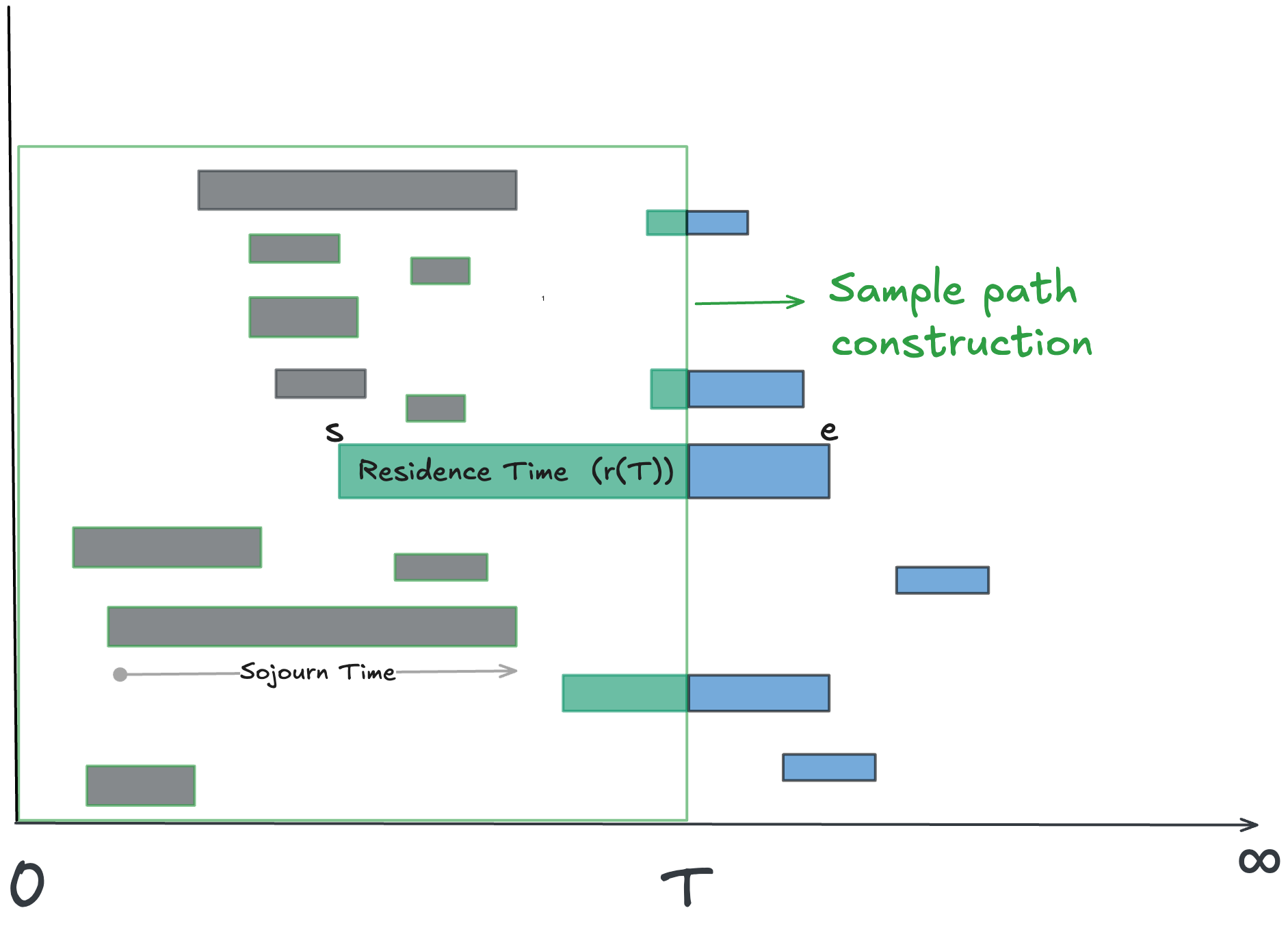
Sample Path Construction for L=λW
It is useful to have a dedicated mental picture of domain of L=λW: an MPP with boxcar functions as marks.
This special case is shown in the figure below and it is intuitively very easy to understand because it a direct representation of the traditional queueing theory model of arrivals and departures from queues (even though queueing is not the focus of the analysis).
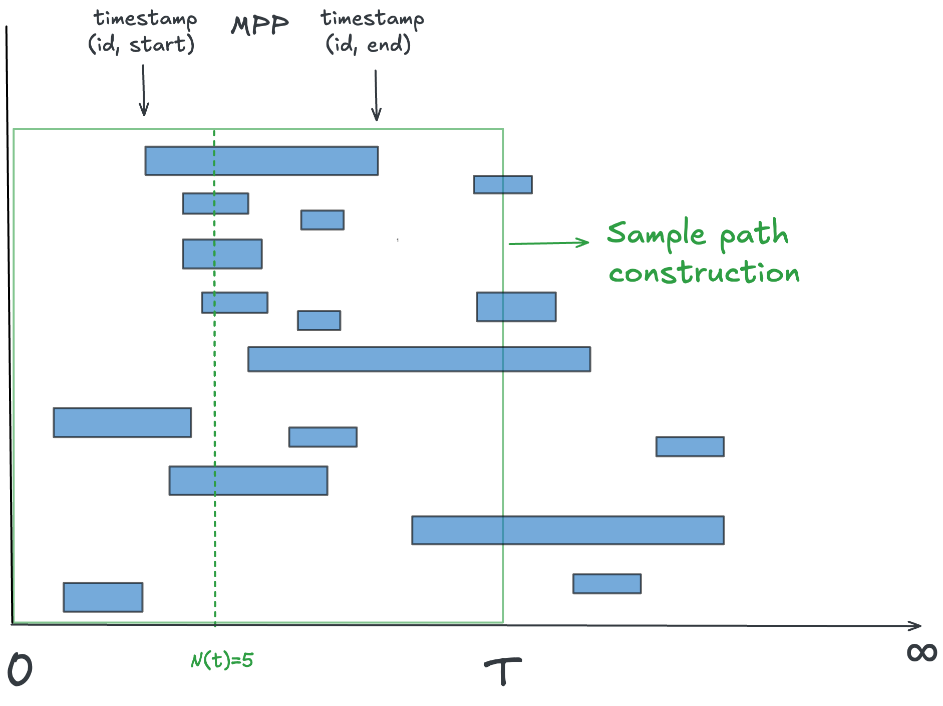
Each element i has a start time 𝑠ᵢ and an end time 𝑒ᵢ (possibly -∞ or + -∞ if start or end times are unknown). An element is called open if its end time is unknown and it is called closed if both start and end times are known.
An element is active at time t if it’s start time is at or before t and its end time is strictly after t. Elements whose end time lies at or before time t are called inactive at time t. Additionally, an open elements is considered active at all t after its start time.
We can extend these definitions to finite observation windows [0,T], where T is implicitly taken as the reference time for determining which elements are active or inactive 11.
Processes and Sample Paths
Sample path analysis focuses on processes defined over an MPP.
A process12 is any time-varying function that we can evaluate over an MPP.
A sample path is the sequence of values we observe when we apply that function to the MPP 13.
For L=λW, the process of interest is the counting process over the set of active elements at a point in time.
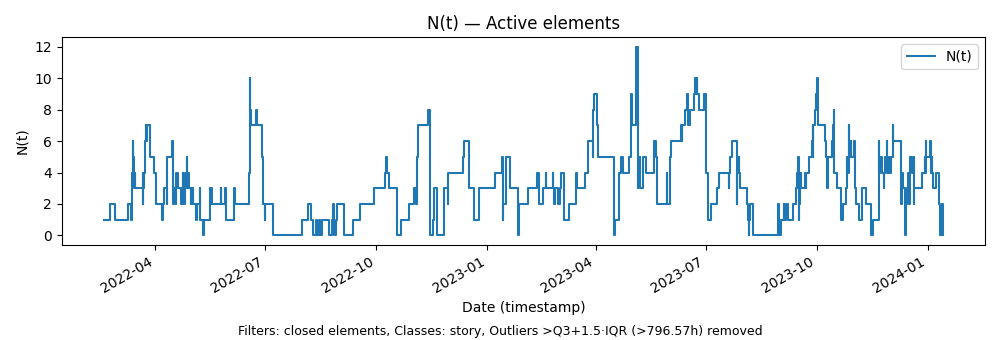
N(t) is the count of active elements at time t 14. The trace of values of N(t) over time, is the sample path of the process N(t).
For the Polaris case the process N(t) counts how many product or customer outcomes are active at time t: elements for which work that has started but has not yet reached a resolved outcome.
In the examples below we will focus on the closed elements in the process - ones for which both start and end dates exist in the data set. It is easier to demonstrate core concepts with this subset first and see how things change when we add open elements into the mix. This is precisely the difference between analyzing the history of the process vs real-time analysis.
The figure below shows this sample path for closed elements15. You can see the characteristic rhythms of our work from moment to moment: bursts of parallel activity, quieter lulls, and variability that reflects customer feedback cycles and the adaptive nature of our small-team process.
The Finite Version of Little’s Law
Any sample path that we observe is finite. One of the most powerful tools that sample path analysis gives us is a version of Little’s Law that applies to any such path at any point in time. Unlike the steady-state, asymptotic version of Little’s Law that gets the headlines, this version is a universal invariant that holds unconditionally16 .
The invariant is expressed as an equation involving three functions of time, derived from the process N(t). Given a sample path over the interval [0,T] these are
L(T): the time average of N(t) over [0,T]
Λ(T): the cumulative arrival rate over [0,T]
w(T): the average residence time over [0,T]
We will define these terms formally and show how to measure each one shortly.
The key point to note here, is that finite version of Little’s Law says that these three functions are always locked together at every point in time by the invariant
Stidham’s sample path proof defines the three quantities in the equation L= λW as asymptotic limits of these three functions,
He showed that if the limits λ and W are well-defined and exist then the limit L is well-defined and exists, which allows us to establish that L= λW holds at those limits.
In this section we will show how to measure the key terms in the finite invariant given the sample path and validate that this invariant holds for our data set. Later, in the section on convergence, we will look at the question of establishing limits and consider the question of how we can verify whether L= λW for a given process.
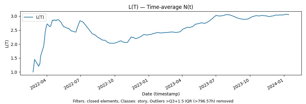
Measuring L(T)
We begin by measuring a quantity L(T) which is the time average of the area under the sample path. L(T) is the quantity from which we derive the left hand side of Little’s Law.
This area is given by
represents total accumulation in units of element-time, over the interval [0,T].
Since each element contributes one unit of time for every unit of time it is active, H(T) is also the total time accumulated in the observation window [0,T] across all elements. This includes contributions from elements that are still active as well as those that are inactive.
To turn this into a time-average, we divide this quantity by the length of the interval T.
This value, in units of elements, is the time-average of N(t) over any finite length sample path up to the time T.
Here is what this looks like for our data.
There are several points to note about this chart:
The “WIP” in Little’s Law.
N(t) tells us how many elements are active at a given moment. L(T) is the time-average of those values measured over the sample path. It is L(T) the time average, that corresponds to “WIP” in Little’s Law, not the instantaneous value N(t)17. Mathematically L(T) is a very different quantity from N(t) and much of the confusion about Little’s Law arises because the two are treated interchangeably in many popular treatments of the law.Stability
The time-average L(T) is bounded but drifts and fluctuates as the process evolves. This is what defines a convergent convergent process that has not stabilized over the entire observation window : the average never settles to a single stable value but stays bounded. By contrast, in a stable process, L(T) may wiggle early on but eventually stabilizes around a fixed long-run average - the limiting value. In a divergent process, the average grows without bound, and no such limit exists18.For flow processes in complex adaptive systems, this behavior is quite common. In this case we are observing the interactions between the product team and the customers developing a new product, and across this boundary the future often does not resemble the past. Instead, the sample-path average keeps absorbing new information from process states that were absent from prior history. The process remains in flux as it responds to a changing environment, and internal adaption19.
In general, its future trajectory is unpredictable though we can get a clear sense of movement and direction from the sample path observed so far. This is the principal benefit that sample path analysis provides in this setting.
Smoothing effect of averaging.
The variation in L(T) is much smaller than the variation in N(t). This is expected: averaging the area under N(t) over larger and larger time windows smooths out fluctuations. But precisely because of this smoothing, even small changes in L(T) over long sample paths are significant. They indicate that new behaviors have appeared in the underlying MPP, altering the long-run average relative to the history observed so far. You can see this visually in the shape of N(t) early in the history vs later in the history, but L(T) captures this quantitatively 20.
L(T) is the lynchpin around which Little’s Law revolves. Given a sample path, we can always measure L(T) exactly: it is simply the time average of the number of active elements over [0,T] as computed above.
But on the right-hand side, the situation is different.
Measuring Λ(T)
In our MPP, if we focus on the just the sequence of start dates that gives us another point process, which we will call the arrival process. It has an associated counting process21.
Here A(t) gives the cumulative arrivals up to time t 22.
Analogous to L(t), let’s define the cumulative arrival rate over a finite window [0,T].
This is the average rate of arrivals in units of elements per unit time up to T. Here is what that looks like for our data set.
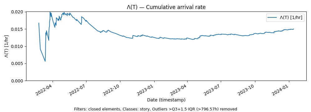
Stabilization behavior.
Λ(T), the cumulative arrival rate, fluctuates sharply early in the sample path as averages stabilize and gradually smooths out as the observation window grows. This is expected: short horizons are dominated by a few arrivals, while longer horizons average out the noise.Stability
Even as Λ(T) smooths with time, it does not settle on a single constant value. Instead, it drifts: high arrival intensity early on, a gradual decline through the middle portion as the average converges, and a modest upward trend in the late portion.Nevertheless, there is a period in the early part of 2023 where the arrival rates converge to values and stays relatively flat before resuming a new trend. This is an example of meta-stable behavior in this parameter.
This is exactly what we should expect from a complex adaptive system. The goals we pursue are neither purely exogenous nor purely internally generated: they are shaped by signals from the market, by customer needs, and by internal adaption from feedback and learning. The arrival process adapts continuously to these forces, and that adaptation leaves its imprint on the observed arrival rate.
Operational implication.
Because Λ(T) still changes slowly over long horizons, even small shifts carry meaning. They indicate sustained changes in the pace at which work is arriving—whether due to customer demand, or the decision to start things internally and pursue more goals in parallel.
Measuring w(T)
The final quantity in Little’s Law is W: the long-run average of the time between start and end timestamps across all elements. In classical queuing theory, this duration is called the sojourn time, a term we will adopt as well23.
In our case study, sojourn time is the critical time to value metric that we are interesting in optimizing our processes for.
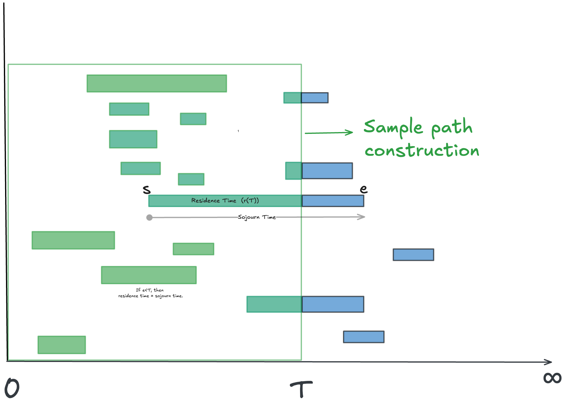
When constructing the sample path over a finite observation window, some end times may fall outside the window. In that case, we only observe part of the sojourn in that window. We define the residence time of an element in [0,T] as the portion of its sojourn time that lies within the window [0,T]. In figure 7, the green shaded areas represent residence times.
It represents the portion of the sojourn that we have observed at a point in time in the sample path, with the remainder representing a (potentially unknown) future evolution of the path at that point in time. In a real-time measurement, residence time represent what we know about the time accumulation in the process up to the point of measurement 24.
Formally we can define the residence time of element i for the window [0,T] as
where 𝑠ᵢ and 𝑒ᵢ are the start and end time stamps for element i.
If both the start and end timestamps for an element fall within [0,T], then residence time equals sojourn time. In general residence time for any element is at most as large as it’s sojourn time.
The average residence time over arrivals up to time T, in units of time units per element, is
This is simply the sum of the durations of the green areas in the figure divided by the number of elements that overlap the window [0,T].
For a deeper dive into the significance of residence time in flow processes, please see our in-depth post:

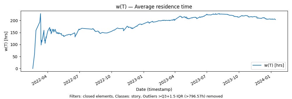
Let’s see what residence time looks like for the Polaris data set.
A few points to note about this chart:
We see the same non-stationary behavior as with the other two parameters: early volatility due to transient effects followed by gradual stabilization, though the overall average drifts upward over time.
The overall trend is a significant increase in average residence time across the history. Even small increases are meaningful when we are dealing with sample path averages, and here we see roughly a 50% increase: from about 6 days in the early portion to about 9–9.5 days in the later portion.
If Little’s Law applies (as we will see it does in this case) these average residence times are the same as the average sojourn times, so we can treat these residence times as our operational metric for time to value.
In absolute terms, these are still relatively moderate numbers for a measure of time-to-value reflecting our generally reactive mode of operation. Interpreted as the average time to realize customer or business-facing outcomes, 6–10 days was an acceptable number for us. But relatively speaking our process “slowed down” significantly over the period we examine.
Residence time reflects the accumulated time of both inactive and active (aging) elements.
Inactive elements contribute to residence time in [0,T] only until its end date, after which their contributions stop.
Active elements continues to accumulate residence time linearly until their end date is reached. The accumulated residence time up for an active element to a given T is the age of the element. If the end date is unknown, these elements accumulate residence time indefinitely.
This clearly shows that convergence of the average residence time w(T) to a finite limit is entirely driven by the balance between active (aging) and inactive (completed) work—precisely in line with well understood flow management principles.
The difference is that the average residence time captures the effect of this balance in a single number, measured consistently over the same window as L(T) and Λ(T) and derived from the same underlying quantity H(T): the total time accumulation in the window.
This is why measuring w(T) is superior to tracking the average sojourn time of inactive elements and the age of active elements separately, as is common industry practice today25 . As we shall soon see, in software environments, where non-stationarity is the rule, residence time provides a superior metric for reasoning about time accumulations in the long run.
The impact of variability
In figure 9 we show the scatter plot of sojourn times overlaid on the average residence time on the sample path. We can see the average residence time conceals a very high variation in sojourn times. In our case it was because we had goals that took significantly smaller, and significantly larger amounts of time to complete. This variability reflects the increasing mix of customer dependent delays vs things that were under our control the more we tested the market.
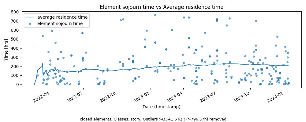
For now, it’s important to keep in mind that variability in sojourns is itself a key operational metric. Even if it’s not always under our control, it determines how long it takes for w(T) to converge in the long run (assuming it converges at all).
Little’s Law doesn’t speak to this convergence speed—it only requires the limit, not how quickly you approach it. But operationally, variability is what governs the “patience” you need before the the data stabilizes in meaningful ways so you can analyze patterns.
In practice this means that we might need to experiment with raw data to remove extreme outliers to get a sense of this convergence - this process requires a bit of judgement and nuance, but it also gives us a good way to operationally distinguish routine variation from exceptional variation26.
We’ll have much more to say about how to reason about this variation for non-stationary sojourn times in later posts.
Value vs Time to Value
This data set includes both internal and customer facing goals (we were not tracking these separately at the time) but while it is the case that many of the low sojourn values in the distribution were internal because we had fewer constraints, and the high value ones were customer facing, this was by no means universally true.
There were high value outcomes that were achieved in a cycles that lasted less than a day and low value outcomes that took us weeks to identify as low value 27. There are many situations in product development where value and time-to-value are correlated. But in general, we should look at value and time to value as independent quantities and be able to reason about both on the same timeline. This is what lets us reason about the relationship between work and value, investment and value etc in a rigorous fashion. This is the motivation for the H=λG form, which we will examine in more detail in later posts.
Putting it together
With all the core machinery for measuring L(T), Λ(T) and w(T) over a finite sample path in place, the finite version of Little’s Law says
for every value T in the observation window [0, T]. This requires no additional conditions, so this is a universal invariant for any sample path N(t).
Let’s prove this. Though the proof is a simple exercise, this finite version is the heart of why Little’s Law is true and it is the most useful operational tool that sample path analysis gives us and it really helps to internalize why it is true.
After we present the proof we will verify that the finite version holds for our sample data set28.
The proof - why the finite version is true
Recall that H(T) the area under the sample path from [0,T] was the time accumulated by the elements that are observed within the window.
We can get the same number by adding up the residence times.
So we can write the average residence time as
From the definition of L(T) we have
Lets rewrite 1/T
So now we have the finite version of Little’s Law.
The proof itself is straightforward, but the deeper question is: what does it mean?
The intuition goes back to the simple conservation principle we discussed in The Many Faces of Little’s Law:
The total time accumulated in an input–output system by a set of discrete items, when averaged per item, is proportional to the time-average of the number of items present in the system. The proportionality factor is the rate at which the items arrive.
The finite version is just this principle expressed in technically precise terms in the language of sample paths and MPPs. It works because both L(T) and w(T) are different kinds of averages of the same underlying quantity H(T): the total time accumulated by all elements in the window [0,T].
Each unit of time an element spends in the system contributes simultaneously to H(T) and to the count N(t).
Once this conservation is recognized, the rest is algebra: the finite identity is simply an accounting relationship about time accumulation.
This also explains why the general version H=λG holds: the argument is identical if, instead of unit contributions, each element accumulates arbitrary real values over time at every instant it accumulates time (ie it is active).
It is important to note once again that the finite version of Little’s Law in a mathematical invariant representing a physical conservation principle. It always holds at all points for any sample path provided the above measurements are made correctly.
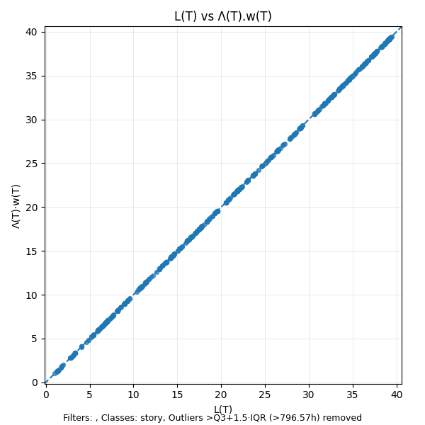
We can visualize this fact using a simple scatter plot of L(T) vs the product Λ(T)·w(T).
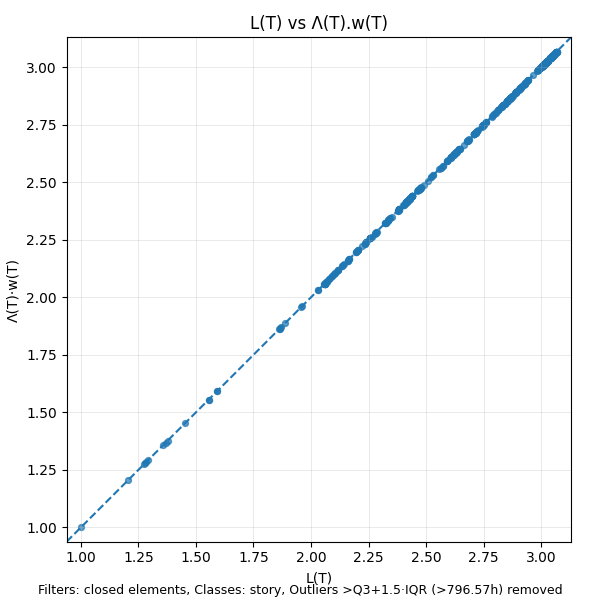
The points on this scatter plot will always lie on the x=y line. If they don’t your calculations are wrong.
In addition to validating the consistency of the measurements, this plot also gives some sense about the distribution of the values of L(T) over the sample path: denser clusters of values represent states that the process returns to very often and represent dominant modes of operation: here we see the numbers largely range between 2 and 3 29.
What is clear is that these numbers move in lockstep and when viewed across the time line these relationships provide rich insights into the long run behavior of the process. The most powerful of these is the ability to reason about cause and effect when we see a change in L(T).
Reasoning about cause and effect
The most fruitful way to look at the finite sample-path parameters L(T), Λ(T), and w(T) is to see how they move together in lockstep when any of the averages change.
This is how Little’s Law should always be read: not as three independent numbers, but as three values derived from the same sample path, bound together by the finite identity.
There is a well-defined causal mechanism embedded in the invariant. Even though the law is written as an equation, the relationship is unambiguously causal.
L(T) cannot change independently.
Any change in L(T) is entirely attributable to a change in Λ(T), w(T), or both, and the magnitude of the change in L(T) is exactly accounted for by the magnitude of the change in the product Λ(T).w(T).
As discussed in The Causal Arrow in Little’s Law, this is also the only kind of cause-and-effect reasoning we can do with these quantities.
This is a direct consequence of the deterministic proof of the finite version of Little’s Law we derived above. Its clarity comes from the fact that the finite version is an accounting identity involving averages, not a statistical correlation or a probabilistic inference.
Let’s take a look at how this type of cause and effect reasoning can be applied in practice. In figure 11 we’ve laid all of the key sample path parameters along the same timeline and we can now look at how changes in values impact each other and how cause and effect can be inferred.
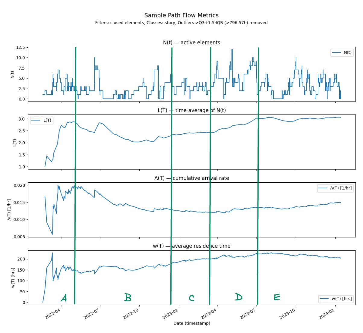
As we look at the sample path and the parameters derived from it over a two year history, we can see distinct shifts in behavior regimes.
Region A (early 2022 – mid 2022):
What we see: L(T) rises steeply, Λ(T) is initially very high but falls quickly, while w(T) rises. In N(t) we see bursts of overlapping work.
Interpretation: Much of the behavior in this early phase are due to transient effects while the averages are still stabilizing. While the finite identity holds as each point in the time, the variation in each value is typically due the fact that we are seeing new states of the system constantly at smaller timescales. Once we have seen “enough” of the history to be representative of the process, the averages settle down into a narrower range even as they continue drifting in lockstep over time. It is usually best to ignore these early segments of the sample path in any sort of cause-effect reasoning.
Region B (mid 2022–early 2023):
What we see: L(T) drifts slightly down, Λ(T) declines further, and w(T) stabilizes. N(t) shows fewer simultaneous elements.
Interpretation: Here Λ(T) and w(T) move in opposite directions: declining arrivals counterbalance stable residence times. The result is a lower, flatter L(T). This is the most balanced operating mode in the history.
Region C (early 2023 - mid summer 2023)
What we see: L(T) starts to climb again, Λ(T) levels off, and w(T) rises steadily. N(t) shows more concurrency than in Region B.
Interpretation: With arrivals steady, the increase in residence time drives the increase in L(T). There’s little counterbalance—w(T) dominates, so L(T) rises.
Region D (summer, fall 2023)
What we see: L(T) reaches its peak, while Λ(T) and w(T) both rise modestly. Yet their simultaneous increases amplify each other, producing a sharp increase in L(T). N(t) shows frequent high-concurrency spikes.
Interpretation: Even small, simultaneous increases in arrivals and residence time compound under Little’s Law. This amplification effect is what drives L(T) to its maximum here.
Region E (winter 2023 - early 2024)
What we see: L(T) stabilizes at a higher plateau, Λ(T) continues a gentle upward drift, while w(T) eases slightly. N(t) shows consistent but elevated concurrency.
Interpretation: Here we see counterbalancing: rising arrivals are offset by easing residence times. The product holds L(T) steady at a higher level, marking a new operating mode.
Overall, we can see that starting in mid to late 2023, the operating regimes started shifting. The main difference is that we had not landed any customers before then and afterwards these shifts were largely driven by new customers with newly discovered requirements, reworking our features after testing with customer workflows etc.. longer latency in response cycles with customers etc. Our internal process which was more or less held constant throughout this two year period. So the shifts here give a picture of the pressure the real world environment in which we were working was placing on us, and how our development process responded to that.
The value of this type of analysis is that we can see the effects of this quite clearly in the finite sample path flow metrics even if we know nothing about the process.
Key insights:
The three metrics are always locked together, but whether L(T) grows or stabilizes depends on how Λ(T) and w(T) interact.
When they move in the same direction (Regions A and D), the effect is amplified in L(T).
When they move in opposite directions (Regions B and E), the effect is moderated.
When one dominates (Region C), L(T) follows that trend.
Either way, by continuously monitoring N(t) and L(T), we can detect shifts in operating regimes as they happen and trace them back to their proximate causes in Λ(T) and/or w(T).
Even though we are showing cause and effect at large timescales in this example, it is important to note that this type of reasoning is possible for changes between any two time points on the sample path, even ones at small scales.
The techniques to do this type of causal reasoning across and between timescales is one of the key contributions of The Presence Calculus. It requires additional machinery, but if you are curious, the details are here. We’ll have more to say about this topic here on the Polaris Flow Dispatch as well in coming weeks.
The impact of process changes
Viewing history consistently along a sample path also makes these measurements useful for validating the impact of larger process changes. For example, if we intervene to reducing process time in the underlying process, we should see meaningful decreases in w(T) and L(T) while Λ(T) remains relatively stable (assuming it holds constant).
In practice, however, shortening residence times often frees up capacity, creating slack which lets you accept more work. In that case, Λ(T) may drift upward, and the net effect on L(T) depends on whether the gains in residence time outweigh the increase in arrivals. Either way, the invariants ensure that the changes in L(T), Λ(T), and w(T) remain locked together by Little’s Law and we will have seen the impact of the change - more slack or greater arrivals at lower residence times.
For changes to show up clearly in these metrics, the interventions must have a lasting impact: incremental improvements that only nudge single metrics at short time scales will typically not register in long run averages 30.
Finally, while the finite version is extremely important for operational measurements, we should always keep in mind that this expresses L(T) as the product the cumulative arrival rate and the residence time over a finite window, while Littles Law as we commonly understand it expresses it as the product of the long run arrival rate and long run average sojourn time.
So we still have some work left after this to prove our case that Little’s Law as we know it applies to complex adaptive systems.
Convergence,Equilibrium and Coherence
Let us now turn to the question of whether L=λW applies to a complex adaptive system such as the one we have just examined.
To review, Stidham’s sample path proof defines the three quantities in the equation L= λW as asymptotic limits of these three functions,
He showed that if the limits λ and W are well-defined and exist then the limit L is well-defined and exists, which allows us to establish that L= λW holds at those limits. Which raises a sticky question - how do we know the limits for limits λ and W are well-defined and exist?
Stidham’s theorem is stated for infinite sample paths, yet in practice we only ever observe finite ones. When proving theorems, stationarity and ergodicity are assumed to ensure the averages converge. But in operations management, we are not proving theorems, we need some direct evidence that limits exist even we cannot observe the sample path all the way to infinity.
In the Polaris data, two years of history showed no sign of divergence (which would have ruled out the limit entirely), but neither did it show clean convergence. Instead, the averages Λ(T) and w(T) wandered in metastable patterns—exactly what we should expect in a complex adaptive system.
So does that mean Little’s Law, L = λW, fails in such settings? The answer is no. The law still holds, but the argument for it requires more nuance than the textbook proofs.
If you examine the Stidhams proof of L= λW the reasoning is as follows: if the limits
are well-defined and exist, then Stidham showed that at those limits the end-effects due to the difference between the cumulative arrival rate and the true arrival rate, as well as the difference between average residence time and average sojourn time vanish. Thus at the limit the quantities in the finite version of the law are identical to those in L= λW, and so the law holds.
Sample path coherence
To quantify the impact of end effects, we define time varying versions of λ an W over an observation window [0, T]:
λ*(T): the empirical arrival rate — the number of elements that became active (arrived) by time T, divided by T. Λ(T) also counts elements that were already active before time 0 (elements with unknown start dates). The difference between Λ(T) and λ*(T) are the end effects for arrival rate over [0,T].
W*(T): the empirical average sojourn time — the total sojourn time of all elements that became inactive by T, divided by the number of deactivations. Sojourns are measured relative to each element’s own start and end, not the observation window. In the figure below the grey rectangles are counted in W*(T) but the green ones are not. w(T), the average residence time, counts both. The difference between w(T) and W*(T) are the end effects for sojourn time over [0,T].
In our case, we are assuming that there were no arrivals before time 0, so the cumulative arrival rate and true arrival rate are the same and there are no end effects on that term. In the example in figure 12 the blue bars represent the end effects for sojourn time vs residence time.
As we discussed in The Many Faces of Little’s Law over sufficiently long intervals, if the process is not divergent then the sojourn times of the inactive elements dominates the residence time of the active elements and the end effects vanish the longer the window we observe 31.
The idea is to check for empirical convergence between the values of L(T) and the product λ*(T).W*(T) over any [0,T]. Equivalently, we can check pairwise if w(T) converges to W*(T) and Λ(T) converges to λ*(T) at each point on the sample path.
The empirical approach bypasses the postulate of the existence of limits in Stidhams proof. Instead of assuming the limits exist, we measure differences
We can set some suitably small convergence threshold and say that the Little’s Law holds approximately at very point in time where the difference is below the threshold.
If they do, then we can assert that
where L(T) is the usual time-average of N(t) over [0,T].
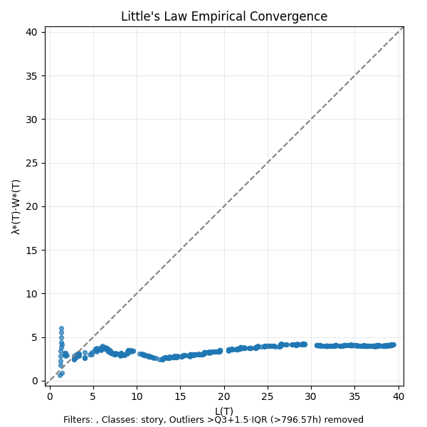
Let’s plot L(T) against λ*(T).W*(T) the way we did for the finite version to see this empirical convergence in action.
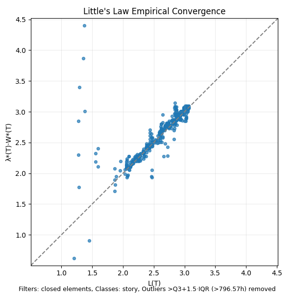
We see that the values stay clustered around the x=y line for most of the sample path. This, in spite of the fact that the averages keep moving around almost all along the sample path!.
We can also directly verify the convergence between the two related quantities on the right hand side directly as well so that we can where this deviation occurs along the time line.
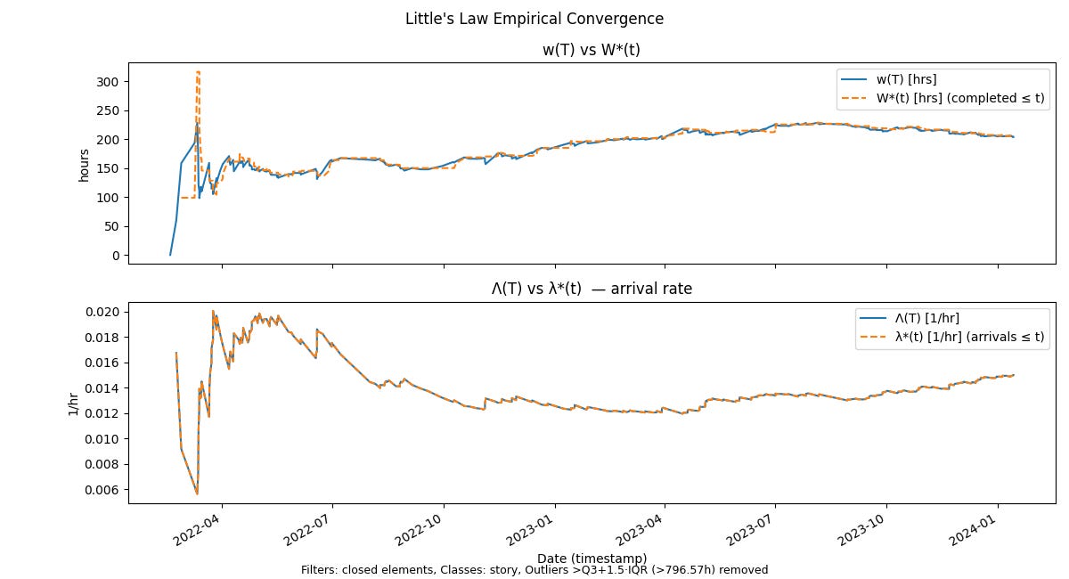
As expected, arrival rates are identical since there are no end-effects in play in our data set, and the average residence time tracks the empirical average sojourn time almost everywhere on the sample path!
So we can say that in this case, even though we are working with a complex adaptive system, the process remains in a quasi-equilibrium state all along the sample path even as the underlying averages move around. Little’s Law continues to hold almost everywhere on the sample path! This may be unexpected, but it is has a direct mathematical explanation.
Why managing age is the key to convergence
w(T) and W*(T) converge if the sojourn times of active elements dominates the residence time as the sample path grows. The gap between the two averages is proportional to the contribution of active elements to the average residence time. Intuitively, this contribution is the sum of the green bars in Fig 12, the total age of the active elements in the observation window.
If that total age grows more slowly than the length of the observation window, the end effects disappear and the two averages converge over longer and longer windows.
This gives us a clean operational check for convergence. The total age of active elements along the sample path must grow sub-linearly as the window is extended longer and longer. If it does, the process tends toward convergence; if it does not, the process tends towards divergence.
Typically, the gap between the curves grows when you have many open elements (with no end date), heavy-tailed sojourns, or long bursts of arrivals that lets the total age of active elements grow linearly with T rather than sub-linearly. Convergence will be slower or impossible in these cases and the cloud will spread farther from the x=y line. That’s a signal that L=λW does not hold.
Divergence
Its not hard to see divergent behaviors emerge even in the Polaris data set. All you have to do is to include open elements (with unknown end dates) into the calculation. We had explicitly ruled that out in our earlier analysis by only including closed elements in the data set - elements with known end dates.
In this case Λ(T) remains bounded but w(T) grows unboundedly. This corresponds to the scenario where certain elements never become inactive once they become active and continue accumulating residence time proportional to the size of the observation window.
Operationally when residence time starts to diverge, it is a signal that there are aging elements in the process that we need to pay attention to - this is perfectly consistent with the principles we use today in managing flow.
But there are two keys things to note;
The finite identity L(T) = Λ(T). w(T) holds regardless of whether the process is convergent or divergent. You can see this in the scatter plot below for the divergent process above.

Fig 16: The finite version applies even to divergent processes In the case of the divergent process not only is L != λW in the limit but the values in the finite version and empirical version do not converge. But there is still valuable signal in this fact. See the scatter plot for the empirical convergence below:
This chart is not just a random scatter of points around the x=y line as one might perhaps expect.
The shape of the distribution shows that L(T) and the product λ⁎(T)W⁎(T) diverge early and then follow largely independent trajectories. But there’s clear structure there: the left hand side L(T) continues to grow, while the right hand side stays bounded.
Why? The arrival rate behaves similarly in both formulations, so the difference is driven by the treatment of sojourn times:
L(T) is a time average that includes the residence time of open elements.
W∗(T) is a sample average that only includes the sojourn times of closed elements.
In a convergent process, these differences shrink as T grows: sojourn times and residence times reconcile, and the cloud collapses toward the diagonal.
In a divergent process, residence time grows unboundedly while sojourn times (and arrival rates) remain bounded. The result is exactly what we see here: the “cloud” drifts steadily away from the x=y line.
So even when the identity L=λW fails to hold, the behavior of the system follows the conservation laws of the finite identity and we can still reason about cause and effect in the behavior of arrival rates and sojourn times indirectly.
Equilibrium and Coherence
When W*(T) converges to w(T) it means that the sojourn time reported on average for elements matches the residence time in the system. The process is at or near equilibrium even if the underlying averages shift over time. This makes the finite version, which is simple to reason about an accurate proxy for the element-wise average sojourn time.
Operationally want to report and manage to average sojourn time because this is the externally facing metric, but when the process is convergent these outside-in and inside-out metrics are equivalent. We call this operational coherence. In a convergent process, we can confidently report finite window parameters for this.
This is a key difference between using sample path metrics and flow metrics defined over arbitrary finite windows as is common practice in the software industry. In operations management today, we typically measure flow metrics on finite time windows aligned to business processes and cadences. Sample path metric are aligned to the a single, sufficiently long sample path and reflect the real-time internal dynamics of the process over the long term - they represent the “voice of the process” so to speak32.
In fact the misalignment between the operator time windows used for internal reporting and the sample paths for the underlying processes are a key reason why many operational metrics seen on dashboards today feel noisy and hard to use for making meaningful operational decisions.
Once you start measuring along sample paths the long run sample path metrics don’t change drastically over short operational windows, and when they do, they give you actionable diagnostics on what you should be paying attention to33.
Much clarity ensues once start measuring flow this way.
Does Little’s Law Apply to Complex Systems?
Let’s finally put this question to rest.
All the behaviors we have shown are independent of whether or not the underlying “system” is a complex adaptive system. The same behaviors of transitioning from convergent to divergent behaviors and back can be observed with ordered and unordered systems, linear and non-linear systems, chaotic systems etc under the right conditions.
Little’s Law is not a contingent property of specific systems. It is a universal rate-conservation law, dictated by the mathematics of time accumulated by elements in a process, and it shows up in practice as clear, observable behaviors: convergence or divergence along the sample path in all situations - whether or not the formula in Little’s Law applies.
So yes, we can confidently say Little’s Law can be applied to complex adaptive systems.
The Complex System Advantage
Complex systems introduce more, well, complexity: of system behavior.
They don’t converge quickly to a single stable average value. The averages keep moving around. We cannot guarantee that the finite limits exist. This is why having a powerful piece of mathematics like sample path analysis to reason about how such systems behave over time is so valuable.
On the other hand, in a complex adaptive system we have an advantage: as humans who are part of the system we can closely monitor convergence and divergence trends in real time with this same machinery and adapt to change the trajectory of the sample path!
We don’t always need to limit ourselves to building fully convergent, stable processes, because we are part of the system and have the power to influence convergence and divergence from within the process!
If a process is diverging and we want it to converge we know what we need to act on.
If a process is converging and we want it to diverge (say N(t) represents active customers) we know what we need to act on.
What the machinery of sample path analysis gives us is a mathematically rigorous set of techniques for measuring the drivers of convergence and divergence, the ability to reason about cause-effect relationships between them, and the ability to act on that knowledge.
A rock-solid measurement substrate, which sample path analysis provides, is a pre-requisite for building sound decision-making systems.
As we all know, with humans in the loop, it’s making decisions and acting on the knowledge that is the hard part. But the job does not get any easier if your measurement system is built on weak foundations. Sample path analysis fixes this in many practical operational scenarios.
In my mind this is what we have been missing in operations management in software development since we started measuring and ironically, it looks like the humble formula that that used to tell us how many widgets an assembly line can produce remains a core part of the solution.
What’s Next?
We’ve only scratched the surface of what sample-path analysis can do in software product development and engineering. Here’s my rough roadmap of topics I’m working on and plan to write about in upcoming posts:
Operationalizing sample-path analysis
I’m working on a bare-bones open-source toolkit to generate basic sample-path results directly from CSV files. I plan to extract this from my proprietary platform so others can experiment with their own data in a lightweight way. If you’d like to help test and refine this with real-world use cases, let me know. I’ll move it up the priority list if there’s enough interest.
From raw data to analysis
A systematic guide to taking a raw dataset, constructing MPPs and producing a usable sample-path analysis like the one we showed in this post. In this case study I glossed over a few tricks that make the story much easier to tell. Without them, the picture can be much murkier when running the analysis on raw data. We’ll work through those caveats and what they mean.
Process–subprocess flow relationships
Extending sample-path analysis to study how processes and subprocesses interact. Sample path analysis is fractal and this linkage is critical to push cause–effect reasoning across processes and timescales.
Integration with Flow Engineering
I’ve been exploring how sample-path analysis connects with value stream mapping in my advisory work for some time now. I’m especially interested in collaborating with folks in this space on creating lightweight, bespoke data-backed measurement models that support rigorous constraint analysis and create a consistent measurement system to show the impacts of flow engineering initiatives on operational metrics. Formalizing value models and making them measurable is part of this thread.
Metastable processes and forecasting
Current forecasting techniques in software (e.g., Monte Carlo simulation on short empirical distributions) have well-known limitations. Sample-path analysis gives us tools to build more robust empirical distributions and to detect when they’re no longer representative. We can forecast without appealing to reference forecasts which don’t actually make sense in complex adaptive system. This opens the door to improving Monte Carlo approaches, and even layering bayesian or probabilistic graphical models on top of MPPs to reason about cause and effect across linked processes.
Use cases for L=λW in engineering metrics
Most standard engineering metrics (DORA, code review metrics, flow metrics, etc.) can be derived from a suitably defined MPP and the identity L=λW. Framing them this way brings unity, mathematical rigor, clarity, and systematic cause–effect reasoning to what is today an ad hoc, theory-free landscape of metrics dashboards.
Use cases for H=λG
We haven’t yet shown concrete examples here, beyond broad claims about the “economics of flow.” I plan to start with cost functions, which align most directly with the machinery we already have. Value functions are trickier: they flip the objective from convergence to divergence, and require working in the finite regime where H=λG no longer holds. My current approach leans on value networks and value exchange models integrated with sample-path analysis using H=λG, but there may be entirely different ways to tackle this. Still early days - if this sparks your interest, I’d love to chat.
Refining the Presence Calculus
The Presence Calculus is a unifying measurement substrate that connects these ideas. Built on the foundation of sample-path theory, it extends those concepts to reason and compute efficiently across timescales and across model boundaries. Conceptually, I view sample path analysis as a core analytical technique within the Presence Calculus.
The machinery for sample path analysis we’ve presented here can become unwieldy when applied beyond single processes or across timescales. We need higher-level abstractions to describe process topologies and the relationships between sample-path metrics and finite-window metrics measured over short operational windows.
The Presence Calculus provides exactly those constructs: abstractions with provable mathematical properties that make reasoning about process assemblies simpler and scalable, while maintaining rigor.
Across all of these threads, the opportunity is the same: to treat product development and engineering metrics not as ad hoc numbers justified through appeals to intuition or industry “best practices”, but as precisely defined, deterministic, repeatable measurements over processes emerging from complex collaborations, backed by provable mathematics.
By applying the machinery of sample-path analysis, we can analyze the metastable dynamics of most real-world software and product development processes in much richer detail. Compared to the ad-hoc measurements accompanied by vague hand-waving we use to reason about metrics today, it puts operational reasoning with engineering metrics on a much firmer foundation.
If you are interested in any of these topics and would like to either collaborate or contribute please reach out and connect with me on LinkedIn and let me know what you are working on and how we might work together.
Also please subscribe to The Polaris Flow Dispatch to support this work.
This means the process feeding the system you are studying has a stationary probability distribution but also behaves predictably enough that expected values of that distribution agree with the average values measured when over all possible executions of the actual process. If your process feeds a downstream process, then your process also need to be ergodic in addition to being stationary to apply Little’s Law to that downstream process, and so on.. It’s a very strong set of requirements.
If you have not read that post, it will provide more context for the material here. Many sections of this post refer back to it for more informal background and context. It is highly recommended that you read that post before digging into the details of this one.
I was also bootstrapping from consulting revenues, so needed to see traction quickly to decide whether it was worth investing in a building a new product in this space. Ultimately the answer to this was no at the time, for a variety of reasons. But it took longer than optimal for me to reach that decision.
This is simply how we tracked units of work. Any connection to Agile stories is Jira-induced.
I am fully aware that this runs counter to most “best-practice” advice around maximiizng utilization and keeping everyone busy at all times. The point to keep in mind in this case is that our cycles include the customer and in those cases, we have relatively little control over things that are waiting, and in this scenario, I would argue our approach is the correct answer.
Flow efficiency was not a priority.
This was directly counter to the advice I was giving my clients and still do in their context. The justification is that their problem was different from mine. I still think that traditional flow management techniques are valuable if your software delivery process is your constraint.
But I am less convinced that dividing the “value delivery” problem into improving software delivery followed by improving value delivery is the right answer any more. I am of the opinion that two need to tackled holistically at the level of the “cycles” we will see in this example, and that the techniques we are showing here are the building blocks to figuring out how to iterate our way to the the correct things to tackle for improvement with rigorous measurement and data.
Such scenarios exists even inside internal organizational processes where dependencies, priority shifts, internal competition for resources etc make real-world flow of work messy and unpredictable. We can still fruitfully use sample path analysis in all such scenarios and apply Little’s Law and the analytical tools it brings with it.
It is potentially the basis for a next generation of Polaris as a product, but right now the tooling output shown here only exists to support my advisory work and I plan to release some open source tools to gauge interest in the ideas and see whether anyone will adopt them.
The shift of perspective to thinking about the events themselves vs the cumulative effects of their co-presence in time is the explicit focus of The Presence Calculus, where we build further upon the machinery of the sample path techniques we show here.
Note that the. open/closed designation is element relative - the start or end dates are either present or not in the underlying MPP. The active/inactive designation is time-relative.
The definition of the word process here has its roots in the definition of a stochastic process which is simply a collection of random variables - also functions of time. Sample path were studies as realizations of stochastic processes - think a sequence of coin tosses for a random variable “coin toss” with two outcomes heads or tails.
El-Taha & Stidham define the domain of sample path analysis as “processes with imbedded point processes” - a somewhat ungainly construction, but accurately represents the scope of the analysis.
This is just a fancy way of saying instantaneous WIP, but in doing these types of analyses, it is always important to keep in mind that WIP is not simply WIP. We will generally try and attach semantics to WIP other than #items, because this is always possible.
If you are paying close attention you’ll also see we’ve filtered out some outliers in the data, we’ll explain later why we do that.
We discussed the intuition behind why this invariant holds, and how it relates to sample paths in the The Many Faces of Little’s Law, we will avoid repeating it here and move directly to the more technically precise definitions needed to measure the quantities involved. Reading this material in our previous post is highly recommended as context for much of the rest of this post.
This is a distinction many commercial flow metrics tools, and most people plugging WIP into Little’s Law formulas fail to make. It is a big reason why they find Little’s Law doesnt “apply” to their data.
We discussed this abstractly in The Many Faces of Little’s Law and this is a concrete manifestation of those ideas in a real world data set.
In software products, the fact that the code base is continually changing in response to new requirements is the characteristic adaption mechanism. This is intrinsic to software product development. Other adaptations at the SDLC and product scope level may also be in play, but the code base is the substrate that is continuously evolving and the impact of architecture, quality and maintainability of the code base often manifest as gradual, but perceptible changes in the long run sample path behavior of the product development process.
We can clearly see that L(T) has been climbing steadily, and even though the absolute values are small, these are likely to reflect significant underlying shifts in the process and/or its environment and deserve attention. Little’s Law will tell us where to focus.
Note - we are being intentionally pedantic here - the terminology and machinery of sample path analysis is very modular and precise and showing these terms in a simple example like the one we are analyzing will make it easy to see how we can generalize these concepts very easily to model much more complicated processes.
In our current example, we are assuming that N(0) = 0 ie no elements are in process at the start of the sample path. More generally, some elements may have unknown start times or lie before the observation window. These should be included in the cumulative arrivals as “initial” values. In practice, their effect diminishes as the window T grows, since they are averaged out over longer horizons.
We’ll adopt this terminology to avoid confusing it with terms like lead time, cycle time etc which all depend upon having a specific interpretation of what these time stamps represent. We can think of those terms as different ways of naming sojourn time in a given context.
The difference between sojourn time and residence time and its implications were discussed in The Many Faces of Little’s Law. It is worthwhile reviewing that section for context in what follows.
This is not to say tracking aging of individual elements on a day to day basis is not important, it absolutely is. But for long run averages and reasoning with Little’s Law, residence time is the correct lens.
This is important because traditional techniques for detecting routine and exceptional variation like xMR charts assume that the average is stationary. You cannot apply the traditional Western Electric formulas directly to non-stationary data (See Wheeler - Appendix 3) and in case of complex adaptive systems its not merely a matter of binring the process under control - non-stationarity is intrinsic to the domain.
Unfortunately, we were not tracking this metadata using any formal system at the time, so this retroactive assessment is purely based on my own understanding of the specific context behind the data.
This should be pro forma if you are measuring things correctly. If your measured values for L(T), Λ(T) and w(T) don’t satisfy the equality L(T)=Λ(T).w(T) for all T on the sample path, your measurements are wrong. So this invariant also serves as a consistency check on your flow metrics. It should always be possible to measure them correctly using the definitions we have given here - this is partly why we have described them is full detail.
This is not a coincidence: this is also how the size of our team ranged across the measurement period. There are some interesting relationship to be uncovered here, but they are out of scope for our current discussion, since Little’s Law does not attempt to explain cause and effect beyond the relationship between L(T), Λ(T) and w(T).
Much of the machinery we develop in the Presence Calculus is designed to connect changes in these metrics across timescales so we can both detect changes at short time horizons while also being able to keep track of the long run averages - so we have both leading (but less reliable) indicators for change on shorter timescales balanced by lagging (but more reliable) indicators for change on longer timescales.
Stidham’s proof provides a mathematically precise set of conditions for this, and we will revisit this in a later post where we look at what we need to do operationally to guarantee that this convergence happens. But we don’t need to appeal to that here, we can simply directly measure the difference between the averages directly.
See Wheeler Appendix 2 for more elaboration of this concept. We look at sample path analysis as the technique that is the natural extension to find the voice of the process in his terms. The difference is that we are extending the concept to non-stationary processes, whereas Wheeler explicitly limited his methods to predictable processes. Non-stationary processes are intrinsically unpredictable.
Of course, long run metrics are necessarily lagging metrics and the shorter time scale metric like aging are still required as leading metrics. The mathematics of the relationship between leading and lagging metrics in this domain is one of the key original contributions of the Presence Calculus to this picture.
First, this is an excellent post, as is the series. I'm thoroughly enjoying it.
A comment regarding footnote 26: "This is important because traditional techniques for detecting routine and exceptional variation like xMR charts assume that the average is stationary. You cannot apply the traditional Western Electric formulas directly to non-stationary data (See Wheeler - Appendix 3) (...)"
Much as Little's Law has been misunderstood and your exposition highlights we can put it to use in circumstances typically dismissed, I feel the same applies here, where XmR chart is misunderstood.
Appendix 3 does not state that XmR cannot be applied to non-stationary data. Appenix 3, para 3 states:
> When a process is operated unpredictably the process behavior chart will detect the presence of the assignable causes. Each and every signal on a process behavior chart represents an opportunity to gain more insight into your process (includes a figure with a point outside Natural Process Limit labeled "Evidence of Assignable Cause").
My interpretation of Appendix 3 is that when you have non-stationary data, an XmR will show you data points with assignable causes. And it points out that investigating those data points is worthwhile as it will highlight assignable causes of variability. This seems worthwhile if one would like to reduce variability.
If one uses XmR not as control charts, but as signal detection charts (I think this is a more apt use in non-stationary data like product development), I think they are what enables us to know when a squiggly plot of Sample Path Behavior is stable (XmR shows no assignable cause), meta stable (XmR shows process change every now and then), divergent (XmR never settles), etc.