
Stabilizing Flow with Timeboxes
How Flows Stabilize - Part 2


This is the second part of a two-part series where we apply the concepts of stability, equilibrium, and coherence in flow processes to analyze common software development paradigms.
Together, these two posts show how Little’s Law lets us design enabling constraints with mathematically provable guarantees of convergence and stability in software flow processes.
The discussion builds on our earlier series on Little’s Law, especially the concepts in “Little’s Law in Complex Adaptive Systems.”
In the first part, “How Flows Stabilize,” we examined how the combination of hard WIP limits and response-time SLAs function as enabling constraints, and how Little’s Law guarantees that these will stabilize a flow process over a sufficiently long observation window.
This is typical of teams working with Kanban and its variants, but this work has usually rested on informal appeals to Little’s Law to argue that they stabilize a process rather than with disciplined, measurement-driven analysis of actual processes.
The sample-path analysis technique we used in the first part provides this missing link between theory and practice.
It gives us an algorithm to define and measure flow characteristics, derived directly from the proof of Little’s Law.
It allows us to characterize stability and the mechanisms by which processes become stable mathematically.
It lets us evaluate stability, equilibrium, and coherence for any flow process with precision.
When combined with the mathematical guarantees provided by Little’s Law, sample-path analysis gives us a powerful foundation for operational analysis—one that allows us to reason about cause and effect in process dynamics, and to engineer stability in flow processes through the systematic use of enabling constraints.
Let’s recap how this worked in our previous example.
Team Kanban
We saw the general mechanism of how hard WIP Limits and Response Time SLAs work to stabilize flow in the process for a Kanban team.
The stabilization mechanism works as follows
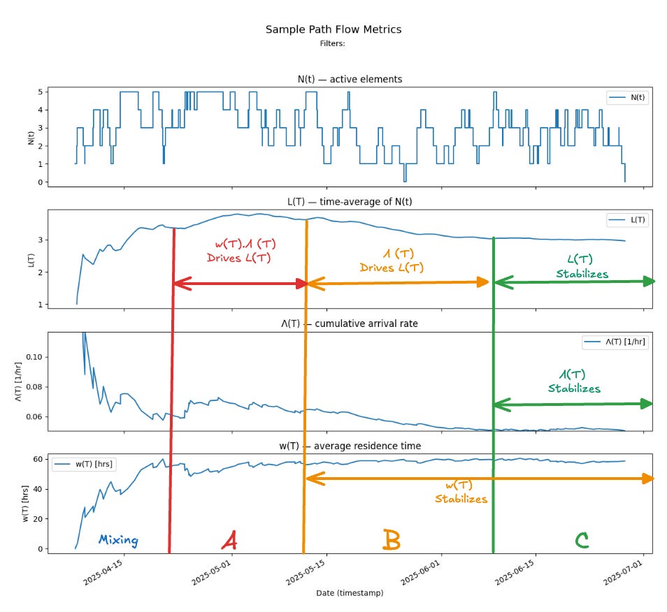
Because the flow process adheres to a hard WIP limit and a hard response-time SLA, the quantities L(T), Λ(T), and w(T) are bounded and, under mild rate-stability assumptions that can be empirically verified, converge to finite limits as T grows.
In Fig 1, the two input parameters Λ(T) and w(T) converge independently to finite limits. Since all three quantities are linked by the finite version of Little’s Law, L(T) = Λ(T)·w(T) at all times, this guarantees that L(T) also converges to a stable limit.
Little’s Law then asserts that the corresponding limit values L, λ, and W satisfy L=λ·W exactly. The latter two — λ and W — can therefore be used reliably as the process’s long-run throughput and average sojourn time.
If you have not read the first part of this series yet, it is highly recommended that you do so to clearly understand the definitions of the terms and the arguments we use above.
We now repeat this analysis for very different type of flow process and see how the concepts translate.
Team XP
This team works very differently from Team Kanban: they collaborate closely with an internal customer, delivering working software increment every single week. Their cadence alternates: one week they ship a meaningful enhancement, the next week they iterate quickly—making smaller improvements, responding to feedback, and fixing any bugs. They respect their iteration timebox strictly, cutting scope if needed to keep commitments within the box.
The working style of Team XP is not one that is typically associated with a “flow process.”
There are no WIP limits.
Work starts and stops at iteration boundaries.
Teams focus on batches of work rather than flow of individual work items.
There are rigid timeboxes.
While timeboxes are considered antithetical to “flow” in some circles, in this post, we will show that in fact, they are very effective at guaranteeing stable flow processes. In a precisely measurable sense, they are more effective stabilizers than WIP limits and SLAs while offering significantly more flexibility in certain contexts.
Sample Path Analysis for Team XP
Let’s start with the sample path flow metrics for Team XP. We have measured the process for 12 weeks so we can compare side by side with the results for Team Kanban.
Recall that we observe the process over a single expanding observation window [0,T] where T extends from the earliest recorded arrival event to the latest recorded departure event.
For each T:
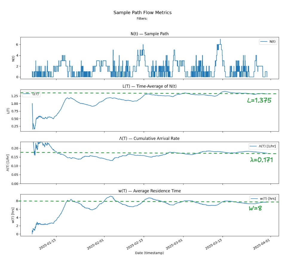
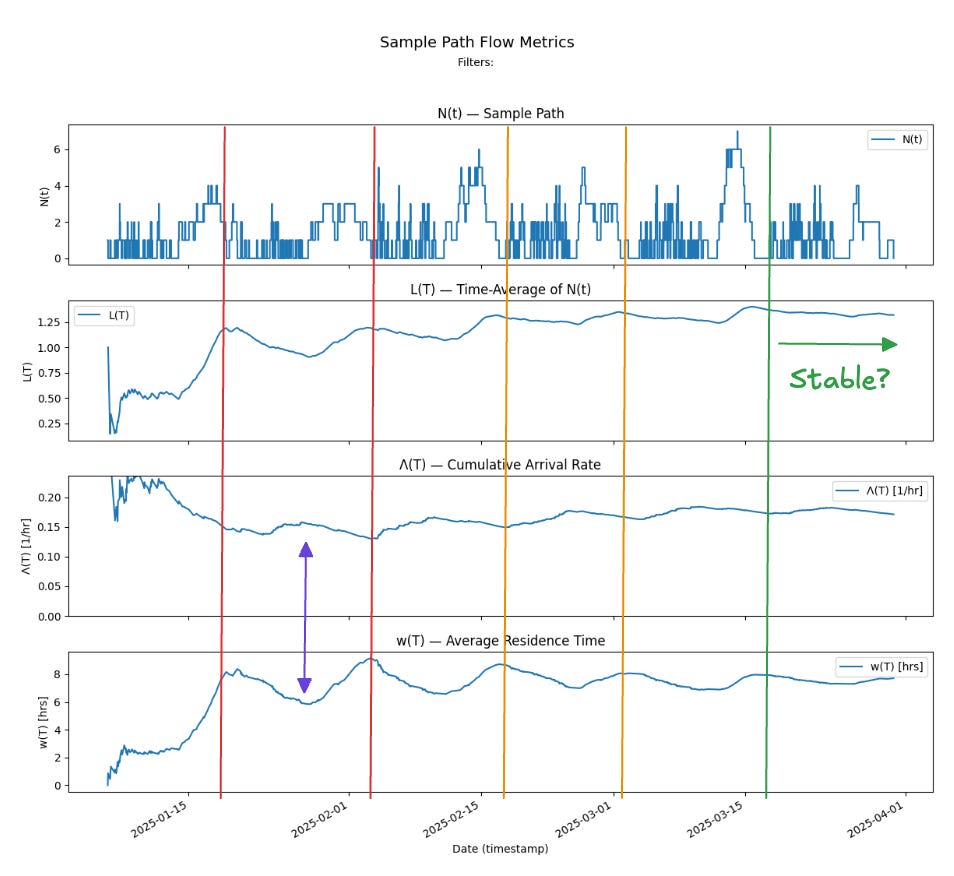
The top chart shows the sample path N(t), which is the instantaneous number of items present in the process (the instantaneous WIP) computed by taking the difference between the cumulative arrivals and departures to the process up to T. We can see the characteristic work cadence of the team XP process here - the alternating patterns where the team works on fewer large items vs more small items.
The next chart show L(T) the time average of N(T) over [0,T]. We can see this time average appears to converge to a finite value L=1.375
The next chart shows Λ(T) the cumulative arrival rate up to T, and this too shows the arrival rate appearing to converge towards the finite value λ = 0.171.
The bottom chart shows the average residence time w(T) and this value appears to converge towards the finite value W=8.
We can verify that L = λW as expected by Little’s Law and thus we can report these three values as the coherent sample path flow metrics for this process.
The timebox as an enabling constraint
If you compare the way the XP process converges vs the way the Kanban process stabilized, you’ll note that there are distinct differences in the underlying mechanisms.
In the team Kanban process, the two parameters Λ(T) and w(T) stabilized independently in time, and once both had converged to a limit, L(T) also converged to a finite limit - the product of those two limits. By the end of the observation window, we could see all values had stabilized to finite values and we could declare the process as stable over the last third of sample path.
In the case of the XP process, both Λ(T) and w(T) converge in parallel to their limiting values and the L(T) appears to converge to its limiting value even before the other two values have fully stabilized.
In fact, the values of Λ(T) and w(T) have still not fully converged to a finite limit by the end of the observation window.
And yet, Little’s Law still holds!
Let’s see why this is happening.
Little’s Law for Timeboxes
In the XP process, N(T) resets to 0 at the end of each iteration, and for many points in between. In understanding how this process stabilizes, we rely on a different mechanism that is embedded in proofs of Little’s Law.
For any flow process measured over an interval where starting and ending values of N(T) are zero, Little’s Law holds exactly1.
This is a very powerful constraint and it impacts the dynamics of the process as a whole in a profound way.
Let’s see how this works.
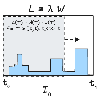
In the figure 3, each iteration represents a timebox.
Provided the sample path N(t) starts at and ends at 0 within the timebox, two conditions hold2.
At any instant inside the iteration, the finite version of Little’s Law holds exactly:
L(T)=Λ(T). w(T) where T is the portion of the sample path from the start of the timebox to some point t within the timebox. Here, Λ(T) is the cumulative arrival rate and w(T) is average residence time within the iteration.
For the iteration as a whole, L = λW holds. Here L is the time average of the number of items, λ is the arrival rate (which equals throughput) and W is the average sojourn time (which equals the average residence time) for the iteration.
Thus at the start and end of each iteration, the process is at equilibrium and the flow metrics for the iteration are coherent.
Now we can see this property holds when we concatenate sequences of timeboxes: since N(T) starts and end at zero for each timebox. So we can claim that for and observation window that starts and ends with any consecutive sequence of iterations, the process is at equilibrium and the flow metrics are coherent.
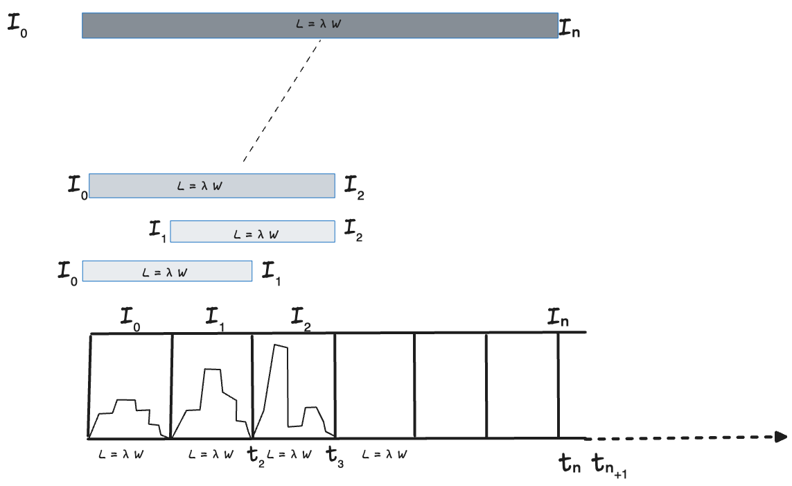
In Fig 4 - even though there may be significant variation of the sample path within each iteration, the process is at equilibrium and the flow metrics are coherent when measured over any observation window that starts and ends at an iteration boundary. This applies to all sequences of length 1, 2, 3 etc.. as shown in Fig 43.
So Little’s Law holds over the entire sample path simply a consequence of the fact the entire sample path is simply composed of a sequence of iterations where the N(t) starts and ends at 0.
So providing you can adhere to a timebox, it serves as a powerful constraint, guaranteeing equilibrium and coherence for sample path flow metrics measured over every observation window that starts and ends at an iteration boundary.
Equilibrium and Coherence
Let’s validate that these claims are true for our data for Team XP.
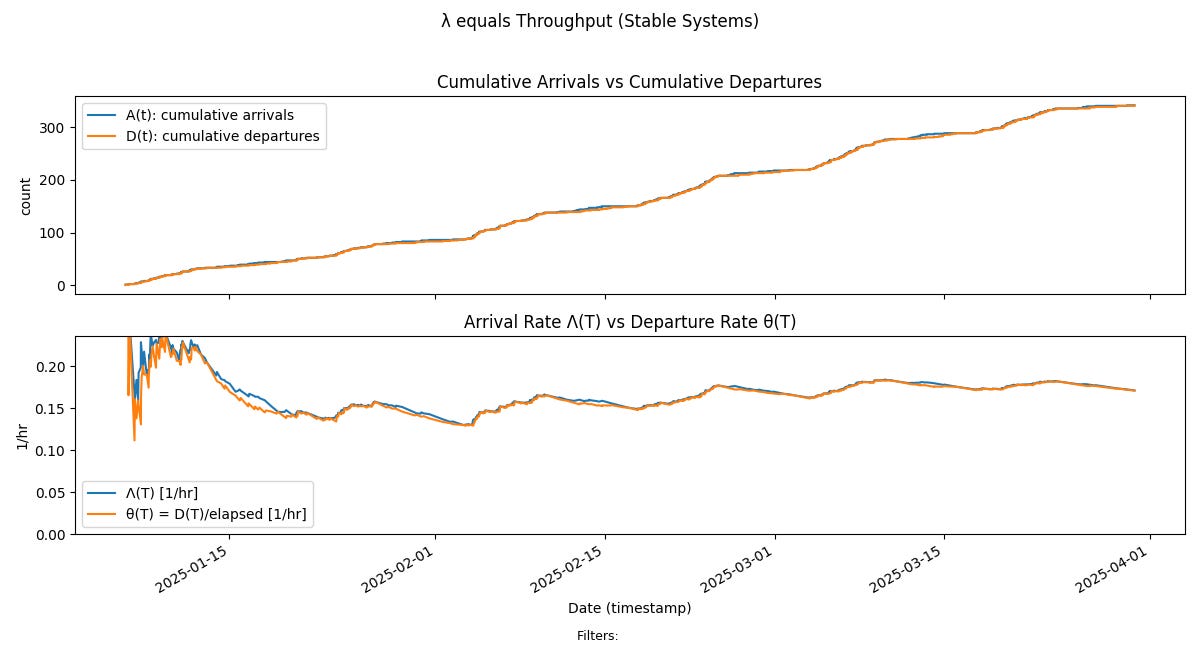
Fig 5 shows that the arrivals and departures are in balance for much of the sample path — a direct consequence of the iterations beginning and ending with zero N(t). Further the arrival and departure rates converge relatively quickly and mostly stay together along the sample path - which means the process is at equilibrium for most of the sample path.
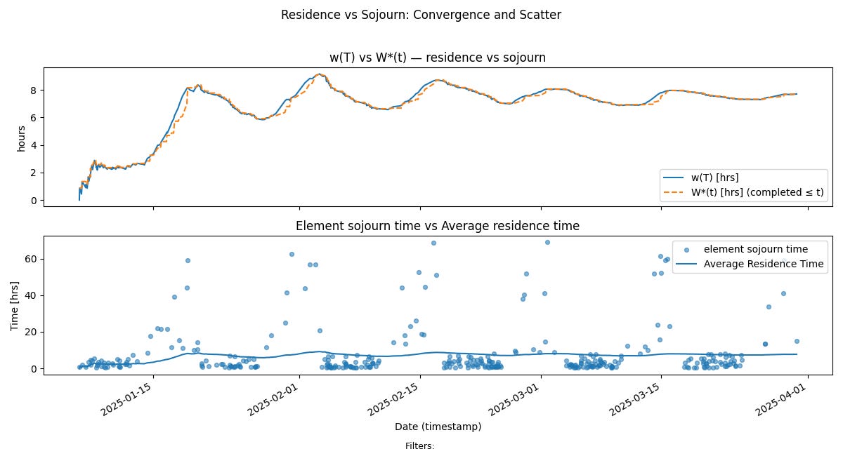
Fig 6 shows that residence time and sojourn time track each other for most of the sample path, drifting apart only during the iterations where items stay in progress for relatively longer period of time.
We can also see that actual sojourn times are evenly distributed around average residence time - making average residence time a good proxy for average sojourn time.
In other words, the process is at equilibrium and coherent for much of the sample path even as the averages along the sample path are not stationary.
So this is a clear demonstration Little’s Law can apply even to processes that are not stationary and this XP process is very good illustration of that fact.
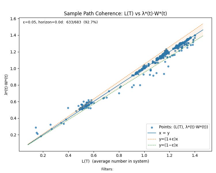
We can summarize all these properties by looking at the sample path coherence plot for the process.
Beginning from a cold start, the process remains coherent and at equilibrium within a 5% tolerance for 92.7% of the points on the sample path!
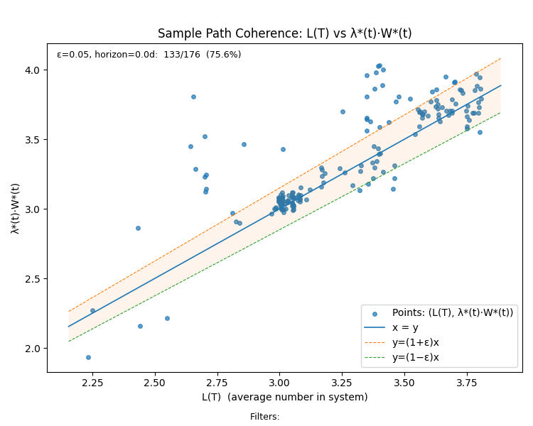
Contrast this with the chart for the Kanban process where only 75.6% of the points on the sample path meet this criteria.
In the team XP case, we can directly establish equilibrium and coherence along the sample path, but we are relying on a different argument from the Team Kanban case to explain why.
In that case we argued that these properties held because the process was stable. We have not argued that here - we showed equilibrium and coherence even without invoking stability.
Which brings up the logical follow-up question4.
Is this process stable?
We have seen for individual iterations, the values of L, λ, and W for the process may change a lot depending upon the workload in the iteration, even if each iteration satisfies Little’s Law.
We still need to determine separately whether or not the process is stable. That is, as we measure over more iterations, we need to prove the values of L, λ, and W converge to stable finite values.
In Fig 8, we see how these averages behave as we take them over longer and longer observation windows. If we look at two consecutive iterations consisting of a week with many small items followed by a week with a few large item, some patterns start to emerge.
Unlike in the Team Kanban case, Λ(T) and w(T) converge in parallel - each getting smaller as we measure over longer intervals, but both exhibit oscillatory behavior.
The alternating patterns of workload across weeks cause Λ(T) and w(T) to move in opposite directions within a 2 iteration window: when the process takes in more items, they complete faster, and when fewer items arrive, they take longer to finish. This inverse relationship creates a natural stabilizing effect—because L(T) is the product of the two, it “settles down” faster than either parameter on its own.
In Fig 8 this manifests as the apparent convergence of L(T) even before the Λ(T) or w(T) have fully stabilized.
But while Λ(T) and w(T) are convergent over the whole sample path, we cannot technically call this process stable yet, since their values never quite stabilize over the whole path.
But timeboxes do provide a guarantee: it can be shown mathematically that a timebox constraint will cause a flow process to converge to stable limits, provided we observe it over a sufficient number of iterations and under mild rate-stability assumptions.
Here’s the reason
The timebox bounds the possible values of w(T): since every work item must start and finish within the iteration, each sojourn time is limited by the length of the timebox.
The timebox also bounds the number of work items Λ(T) that can be accepted and completed within the iteration, given the team’s finite service capacity. Together, these bounds ensure that both the cumulative arrivals and the total residence time within each iteration remain finite.
Because the sample path N(t) starts and ends at zero in each iteration, the area under the curve—representing the total accumulated residence time—is necessarily bounded.
As we integrate this area over larger and larger observation windows composed of many iterations, these bounded contributions yield empirical averages L(T), Λ(T), and w(T) that converge to finite limits.
Even so, for practical purposes we can see that the values we have reported here are stable enough and the fact that Little’s Law applies exactly over the sample path means that these metrics are coherent. So they can still be used reliably as operational flow metrics for the process.
For all practical purposes we have an operationally useful set of sample path flow metrics given this 12 week observation window — the same as in the Team Kanban case.
What does all this mean?
Our main claim is that there are many ways to achieve stable flows. Once we have the machinery to describe and measure what “flow” means independently of the underlying process mechanisms, we can start thinking of flow as a measurable technical property of a process that we can systematically engineer using enabling constraints while designing the process itself to match the context of the complex adaptive system within which it operates.
The two types of enabling constraints - the combination of hard WIP limits and response time SLAs, and timeboxes constitute a complete set of stabilizers for any flow process.
The argument for this is as follows:
If we adopt a policy where we use timeboxes to stabilize flow we can rely on the mechanisms described here to guarantee that the process will stabilize over long enough sample paths. This requires designing processes that periodically reset N(t) to zero by policy.
If on the other hand, our policy the policy is to not require this, then we have to assume N(t) never resets to zero, and in this case - the more general mechanism of hard WIP limits and response time SLAs guarantees stability.
We can use either one independently or in combination.
For example, goal driven processes at the team level can stabilize task level execution using timeboxes. Simultaneously, they can ensure convergence across multiple goals using WIP limits and sojourn time SLAs for goals — the latter facilitating better decision making on how many goals to pursue in parallel when feedback cycles are longer than ideal, and how long to keep individual goals in play if the payoff is smaller than expected.
There is much more to be said about how these enabling constraints can be used to stabilize any given flow process, particularly once you add costs and payoffs to the model, but these are topics for later posts.
The key takeaway from these two posts is this:
Sample path analysis and Little’s Law together provide a rigorous, systematic foundation for reasoning about flow process dynamics and stability.
They give us both the language to define what a stable process looks like, the means to measure whether we’ve actually achieved it, and understand what needs to be done if we have not.
But what about the real world?
There are some obvious objections to all these abstract claims we have made so far, so let’s just put them out there.
In the real world,
Teams don’t stick to timeboxes.
They don’t hold WIP limits or SLAs perfectly.
Work spills over, priorities shift, interrupts happen, work is paused and resumed.
Real flow processes operate in complex adaptive systems, so all these are expected behaviors: by and large, they operate far from equilibrium and stability.
But this is where sample path analysis really shines: by default, sample path analysis assumes a flow process is not stable. It models the dynamics of flow processes that are far from equilibrium using the finite version of Little’s Law as the governing relation on process behavior. Equilibrium, coherence, and stability are measurable states of a process that is expected to operate far from them at most times. It allows us to rigorously study how the process moves between these states.
The stabilization mechanisms we’ve discussed so far—WIP limits, SLAs, and timeboxes—represent idealized process models. They’re the abstract mathematical anchors that real world processes oscillate around. Understanding how these idealized models work through simulations — as we have done here — is a key part of building our intuitions about how flow processes behave.
Depending upon the context, perfectly stable processes may never be possible, nor desirable. The point isn’t that we should expect perfect adherence to an idealized process. It’s that we now have the reasoning tools to understand what happens when we don’t, and these mathematical models give us clear guidance on what is possible.
Flow and stability are not meaningful end goals to be achieved regardless of context. Stabilizing a particular flow process in a larger complex adaptive system might be necessary in order to achieve a particular business outcome, and in this case, the machinery we have shown so far in the series become vital to understanding how to proceed.
For instance if a team works in an iterative process, it is normal for work to spill over across timeboxes. If that team is a critical dependency on multiple teams, and we need the ability to co-ordinate their work with the work of other teams, stabilizing their delivery process is a necessary first step to being able to communicate reliably across teams that depend on this team.
Introducing these enabling constraints — WIP limits, SLAs and timeboxes — as needed, and analyzing their impact on the delivery process for that team using precise measurable definitions brings clarity, rigor and visibility to that process of stabilization.
There are a wide variety of strategies one can adopt to stabilize any given flow process. They are all very highly context specific, and need much more information than is available purely from sample path analysis or the techniques we have shown here.
Having that reference point—knowing what “stable flow” looks like and being able to measure how far away we are from it—is a huge step forward from the informal heuristics and methodology-centric approaches we’ve had until now.
The techniques we have shown here can and should be considered methodology-agnostic tools in a toolkit to manage and improve flow processes in the complex adaptive systems that real world software teams operate in.
We will look at many more of these real-world scenarios in upcoming posts. There’s still a lot to learn about how and where these techniques can be applied, where their limits lie, and how we overlay them on existing ways of working.
This is considered the “easy” case for proving Little’s Law - see for example “Little’s Law on it’s 50th Anniversary”, the survey paper by Dr. Little, Theorem LL.1 (page 537) for an elementary proof.
This follows from the proof in footnote 1.
For a significant generalization of this concept and its application to arbitrary flow process please see the concepts of The Presence Matrix and The Presence Accumulation Matrix in the Presence Calculus.
It’s legitimate to ask why stability matters in this situation. This is a longer topic that we will address more thoroughly in a separate post.
Thank you again, interesting XP analysis.
Two things come to mind at this point in the series.
The first one, is there a third way of working that stabilizes flow? Seeing Kanban explained using sample path analysis, and seeing XP explained using sample path analysis, is there a way to describe yet another way of working working backwards from a stable process into rules that we haven't stumbled upon in the industry yet?
Second, it is all well and good to see these arguments made for L(T), _but_ the business could care less about L(T). The business usually cares about value and other things, along the lines of H(T). So, I'm wondering if any of these Kanban/XP L(T) arguments translate at all to Kanban/XP stabilizing H(T). Yes, I understand Little's Law applies to H(T). What I am wondering about is whether there is a line of reasoning that goes from Kanban/XP constraints -> stabilize L(T) to Kanban/XP constraints -> stabilize H(T). I don't necessarily see why stable H(T) would emerge from Kanban/XP constraints. I think my discomfort comes from f(t) perhaps not being known live/instantenously?
(edit s/Scrum/XP, my bad)