
How long does it take?
Measuring process time in a complex adaptive system


This is the first in a series of posts exploring specific applications of sample path analysis in complex adaptive systems. We introduced this topic in broad strokes in Little’s Law in Complex Adaptive Systems.
In this series of follow-up posts we will dive into specific applications, pointing back to parts of that larger document for more detail and context.
In this post, we’ll look at the problem of measuring process time in a complex adaptive system (CAS) accurately. The conceptual challenge here arriving at a defensible definition of “process time” and a method to measure it, in situations where you cannot always place a firm bound on how long individual instances of a process might take to complete.
This is not a problem unique to a CAS specifically, but it arises commonly when analyzing the dynamics of flow processes in a CAS.
It usually begins with the age-old question..
How long will it take?
The answer is a key input to help guide where we invest time and money in “it”. Even when we have a view of expected payoffs for doing “it”, perceived time and resource commitments heavily shape what gets prioritized.
We know answering this is hard in general because it is hard to predict the future, especially when working in a complex system.
But to even answer the question, we need to answer what might seem like an easier question, but is not always straightforward as it might seem: “how long does it take?”
Examples could be “how long do deals take to close?”, “how long does a feature take to be adopted by 10% of customers?”, or “how long do customer implementations take?”
Given some operational process, all we are asking for here, is a measure of historical process time. Presumably, this should be more straightforward to answer, since it involves no prediction.
This is how we would answer it today:
Identify the operational process of interest.
Observe the process for some period of time (or look at historical data if available) and take measurements for how long instances take complete. Typically this period is aligned to a business reporting window, like weeks, months, quarters etc.
Report some statistical measures on the empirical distribution of process times: averages, percentiles, whatever you prefer.
Continue to repeat the process periodically, and report these measures for the updated reporting period.
This would reported as the answer to “how long does it take?”.
To answer “how long will it take?” you might make some assumptions like: the process time in the future will be comparable to the past, or try and fit a probabilistic model and make forecasts for how long future instances of the process will take to complete.
This is how we do it today: measure the recent past, report the observed process time statistics for a standard reporting period, perhaps create a forecast. Almost all our operational dashboards work this way, no matter what process time we are measuring.
But does this actually answer “how long does it take,” when there is significant variability and uncertainty in process time, or when we cannot reasonably bound process times up front?
Not quite. Not even in theory.
Complex systems are messier
The fundamental problem is that processes in complex systems don’t always have well-behaved statistical distributions. Statistical measures such as averages and variances are not stable, but vary over time. In other words the underlying distributions are not stationary.
Sometimes process times can be consistently bounded, and in such cases, direct measurement over a few weeks is often enough to build a stationary distribution of process time. Such processes do exist even in software development - for example, a software build process, or cycle times in a small disciplined engineering team, delivering changes to production in small batches, with continuous integration and deployment of code.
But they are the exception. Non-stationary distributions, and uncertain process times are the norm for flow processes once we move past the smallest units in an organization, or if the processes involve collaboration across businesses of functional silos within a business.
We are in a non-stationary regime by default in a complex system and here, the measurement window and the thing being measured get tangled when we measure process time.
An example: a sales process
“How long do deals take to close?” seems like a straightforward question. The standard way of answering the question would be to measure and report this on a quarterly cadence.
But some deals close after one demo; others drag on for months. Some begin in one quarter and finish in another. Others span multiple quarters. It really depends on market dynamics, customer demand, specific sales motions in play etc.
No single quarterly “average time-to-close” metric is objectively correct if the question is “how long do deals take to close?”.
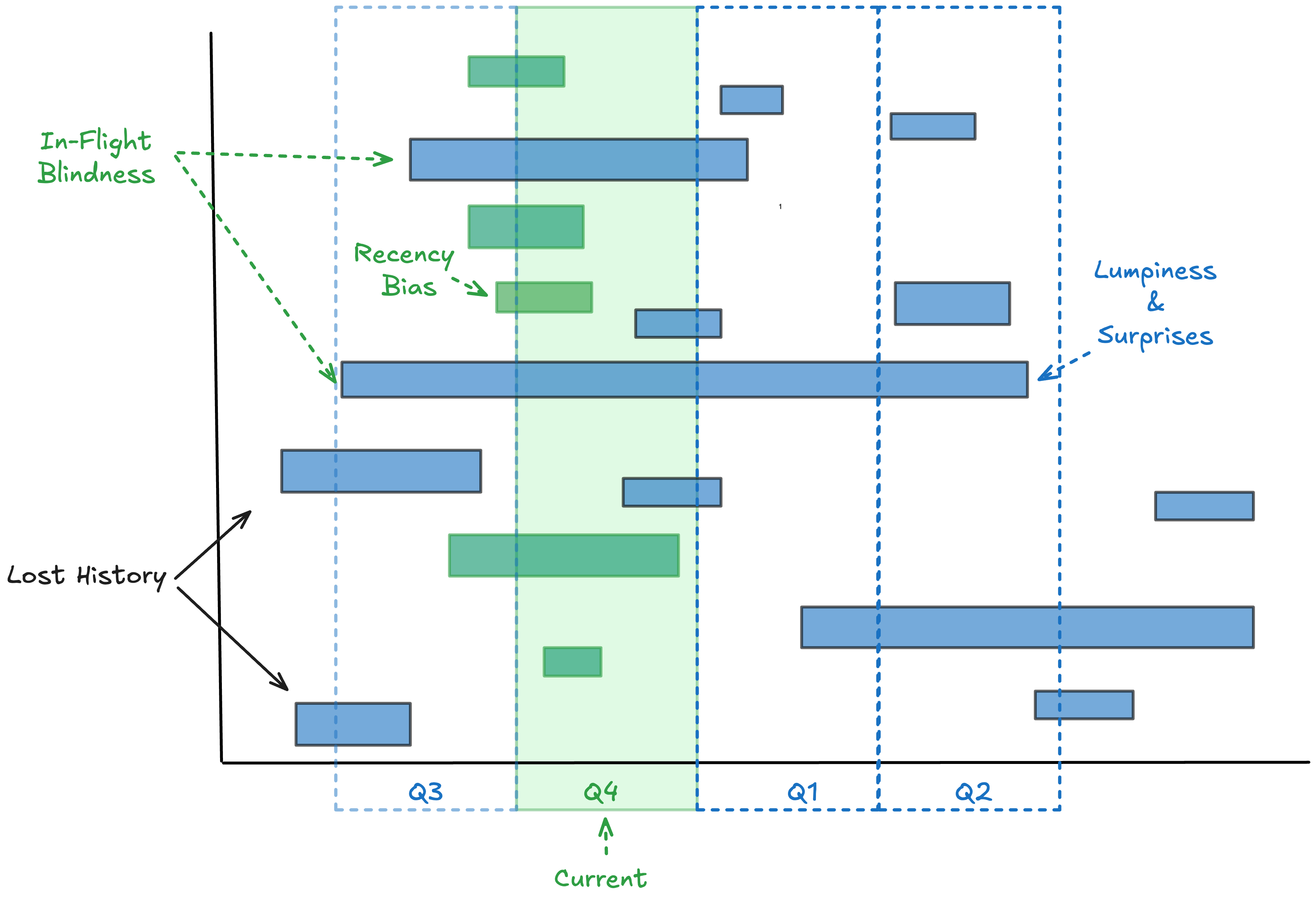
Quarter-by-quarter averaging answers the question “how long did the deals that we closed this quarter take to close?”
Its a very different question and as shown in Fig 1, it produces a noisy, volatile number that suffers from memory loss, recency bias, lagging effects from deals that take a long time to close, and most importantly, ignores the biggest risk items at the time of measurement: the time spent on pending deals that aren’t being counted in the average in the quarter being measured. We are all familiar with the end-of-quarter gymnastics to make the sales “numbers” that results from this strategy1.
“How long do deals take to close?” is a fundamentally different question, and that is the question we need to answer, because it helps us answer follow-ons like:
That’s too long. What can we do to close deals faster?
Are deals taking longer to close over the last six months?
Did implementing the new AI sales tool help us close deals faster?
Is our new sales motion letting us close deals faster?
You can try and answer these questions with the quarter-by-quarter average as your starting point, but it’ll be hard to tell signal from noise. Those numbers are often so volatile that you cant tell how much of it is the true voice of the process 2 vs measurement noise.
Sales is not unique in this.
Delivering a complex software feature touching multiple teams to production,
Contract negotiation or project scope definition between multiple parties,
Measuring adoption cycle time after a new product feature is introduced,
almost any collaborative, process involving independent agents that involves feedback loops and execution risk, shows the same pattern. In other words, most processes in complex adaptive systems.
Reporting process time on a rigid business reporting cadence in such an environment produces plausible sounding statistics, but they are often noisy, and not a robust basis for sound decision making.
Revealing the Voice of The Process
When we working with non-stationary processes Little’s Law becomes very useful.
Contrary to widespread and popular belief even among experts, Little’s Law holds even in processes where the distribution of process times is non-stationary! It is one of the few analytical tools we have that we can reason about the relationship between how averages of distributions change over time without explicitly reasoning about the distributions themselves. And we can do so, entirely deterministically without appealing to any stochastic assumptions at all! This makes it a powerful tool to reason about process time in complex adaptive systems.
Sample-path analysis, which we examined as the core technique behind deterministic proofs of Little’s Law, gives a precise and defensible answer in such situations. It makes some subtle adjustments how we define and measure process time, and in so doing fundamentally solves the problems with finite window sampling we outlined above.
Here’s how it works:
You start observing the process from some fixed starting point in time. This could be a date in the past if you have historical data. Some items may already be in flight; that’s fine, note it and keep going3. The key with sample path analysis is to continuously measure the system for a long time from this starting point4. So rather than observing on fixed width windows, you observe along a continuously expanding window fixed at one end.
As you observe:
Track completed instances and their full durations. These are called sojourn times5.
Track in-flight instances and the time they’ve accumulated so far - this is their current age.
Add them up: this total is the residence time: the time each observed instance has “spent alive” in your window.
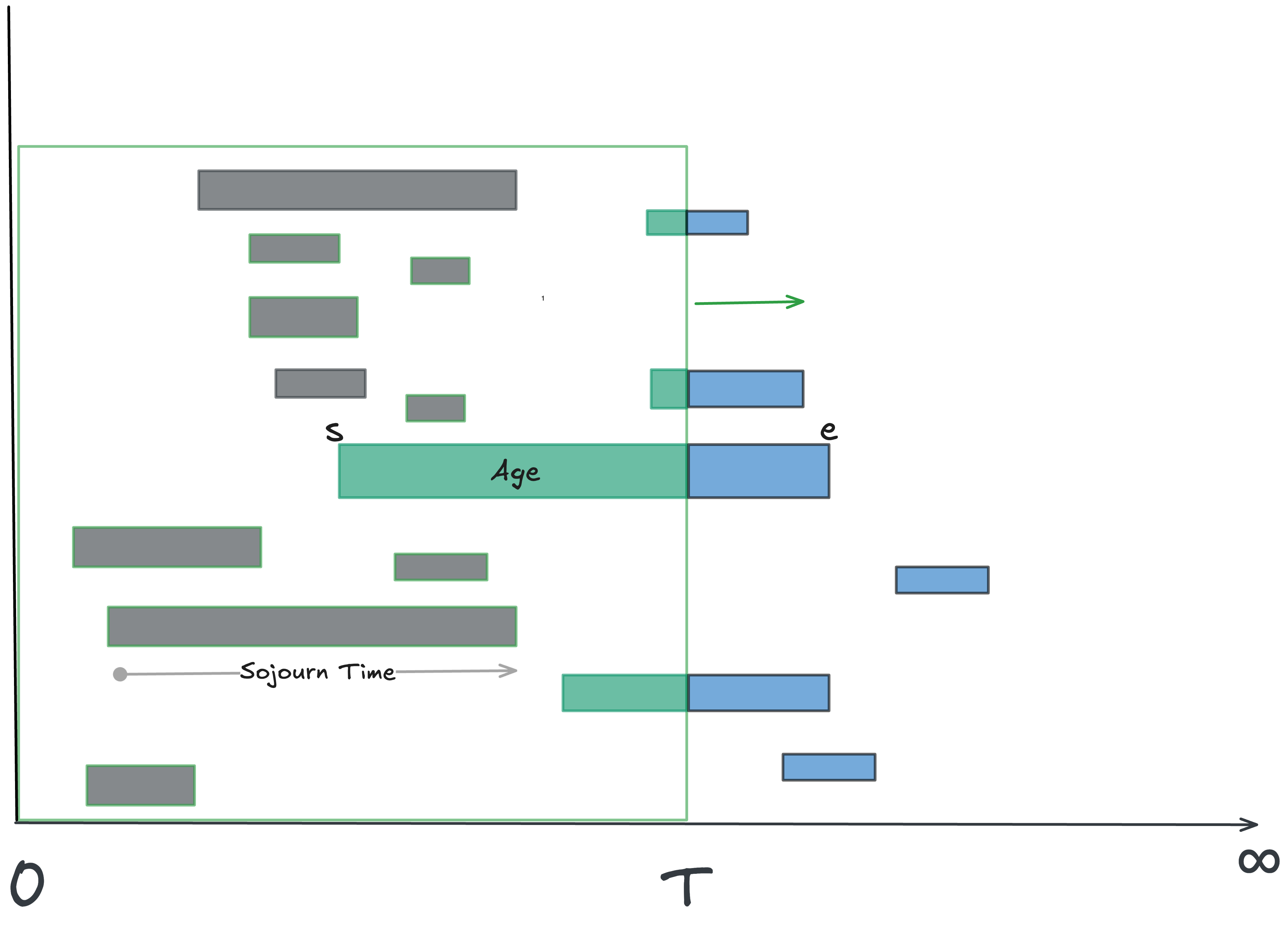
Calculate the average residence time: total residence time across all instances ÷ number of instances observed. In the figure this is sum of all green durations.
To recap there are two possible lenses on process time:
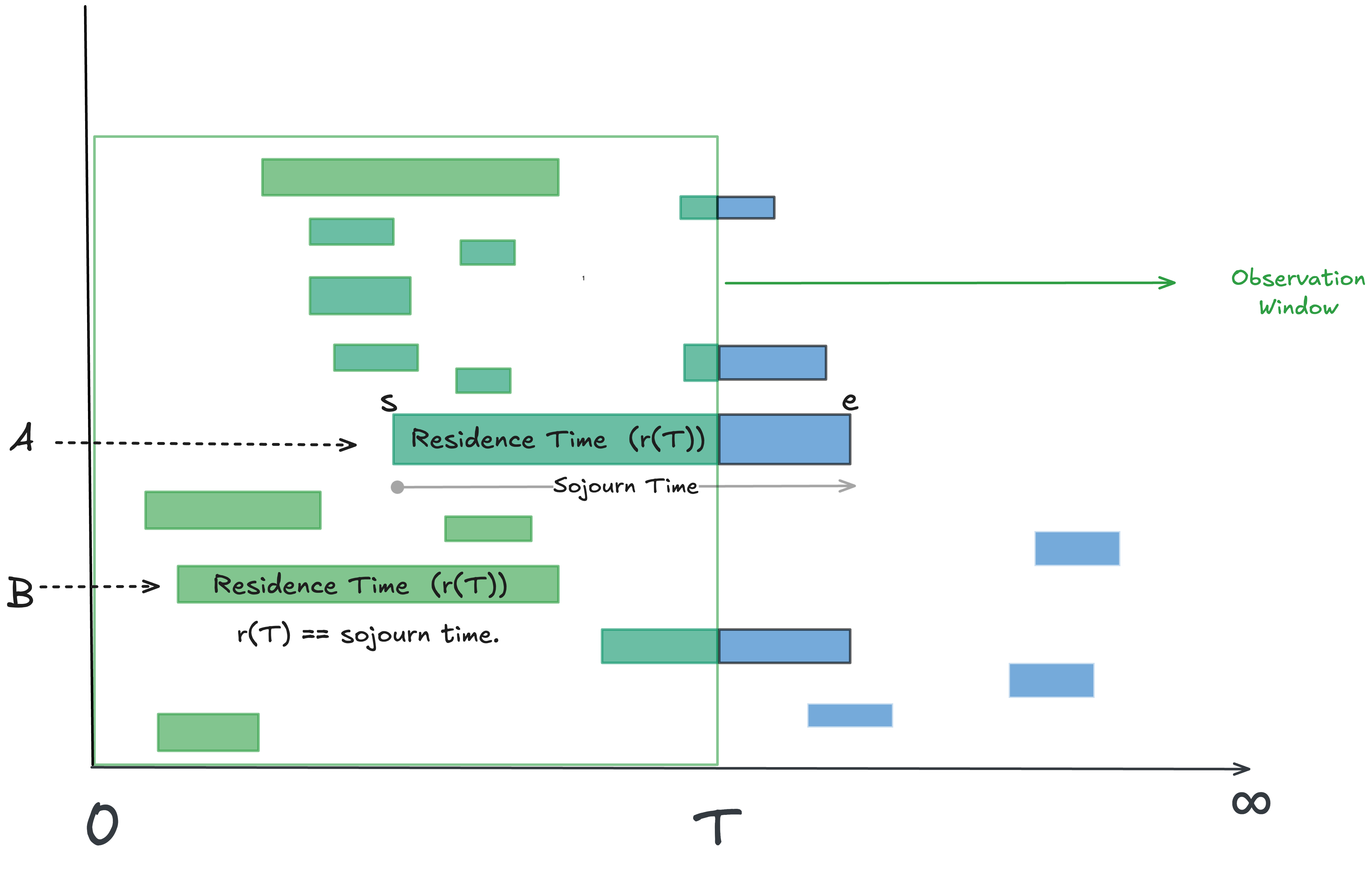
Residence time: total time accumulated by an instance in a finite observation window (all green durations in figure)
Sojourn time: the true start-to-finish time of an instance, only known once it completes. Equals residence time if instance also started in the observation window (instance B in the figure).
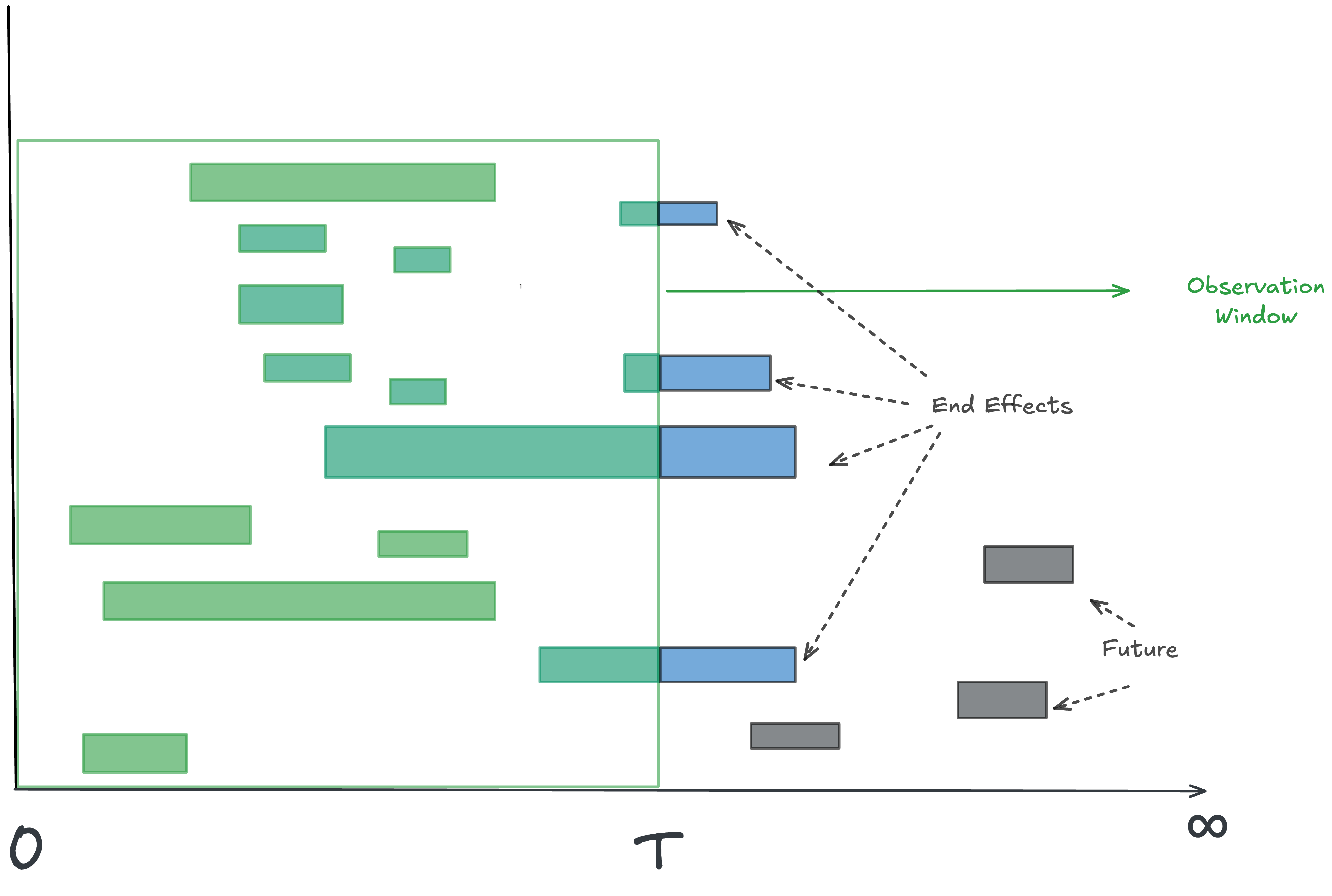
Sojourn time is instance-relative and residence time is observation-window relative. The difference between residence time and sojourn time are the end-effects for the window - the blue bits in the figure 2.
You can think of average residence time as a current estimate of the average sojourn times for those instances that are you have observed so far. But you cannot know the true sojourn time for this window until some point in the future.
This difference between residence and sojourn times is a measure of the epistemic uncertainty6 in your estimate of sojourn times at the moment of measurement.
Where this uncertainty is bounded, we’ll call the process convergent, and divergent otherwise.
In convergent processes, if you observe long enough, the average residence time and the average sojourn time converge. Intuitively, the “blue bits” you haven’t yet seen - the remaining tails of in-flight items - become negligible compared to the total observed sojourn times across all instances in a long enough observation window.
Note that convergence is neither good nor bad. It depends on the interpretation of process time. If the process time you are measuring has a cost it is good for the process to be convergent because we are keeping that cost bounded. If the process time you are measuring creates benefits, economic gains etc. then it is good for the process to be divergent - for example, customer lifetime and the revenues generated over that lifetime.
Ultimately measuring process time matters only as interpreted as a carrier for time-value, whether that is cost, risk, benefit, economic gains etc determines whether we seek convergence or divergence in that measurement.
When does process time converge?
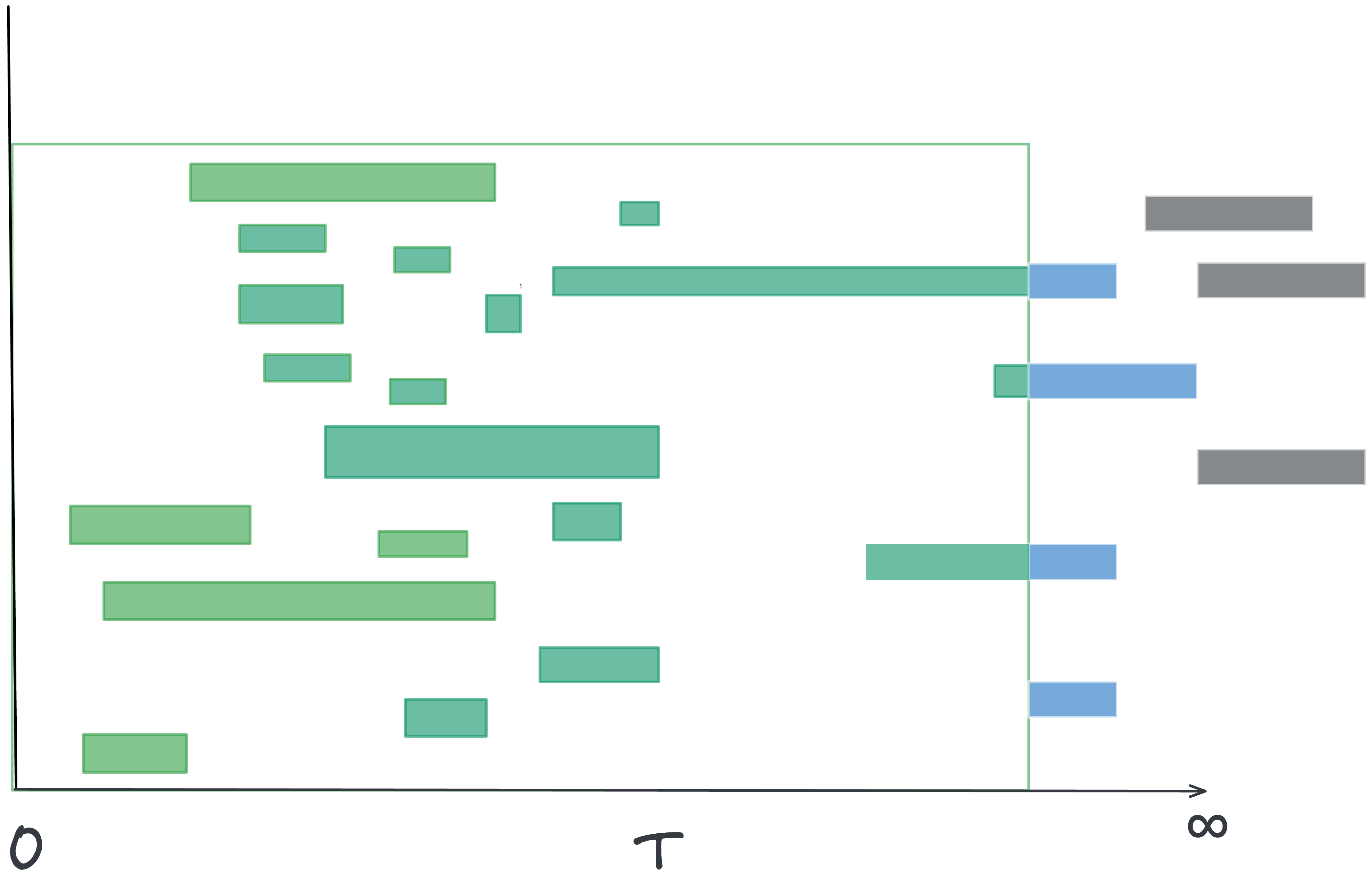
In Fig 5 below we distinguish between the two components of residence time at any moment in time.
The residence time of the completed instances (shown in grey) which are their true sojourn times
The age of the in-flight instances (shown in green) which are only our currently known estimate of a the true sojourn time.
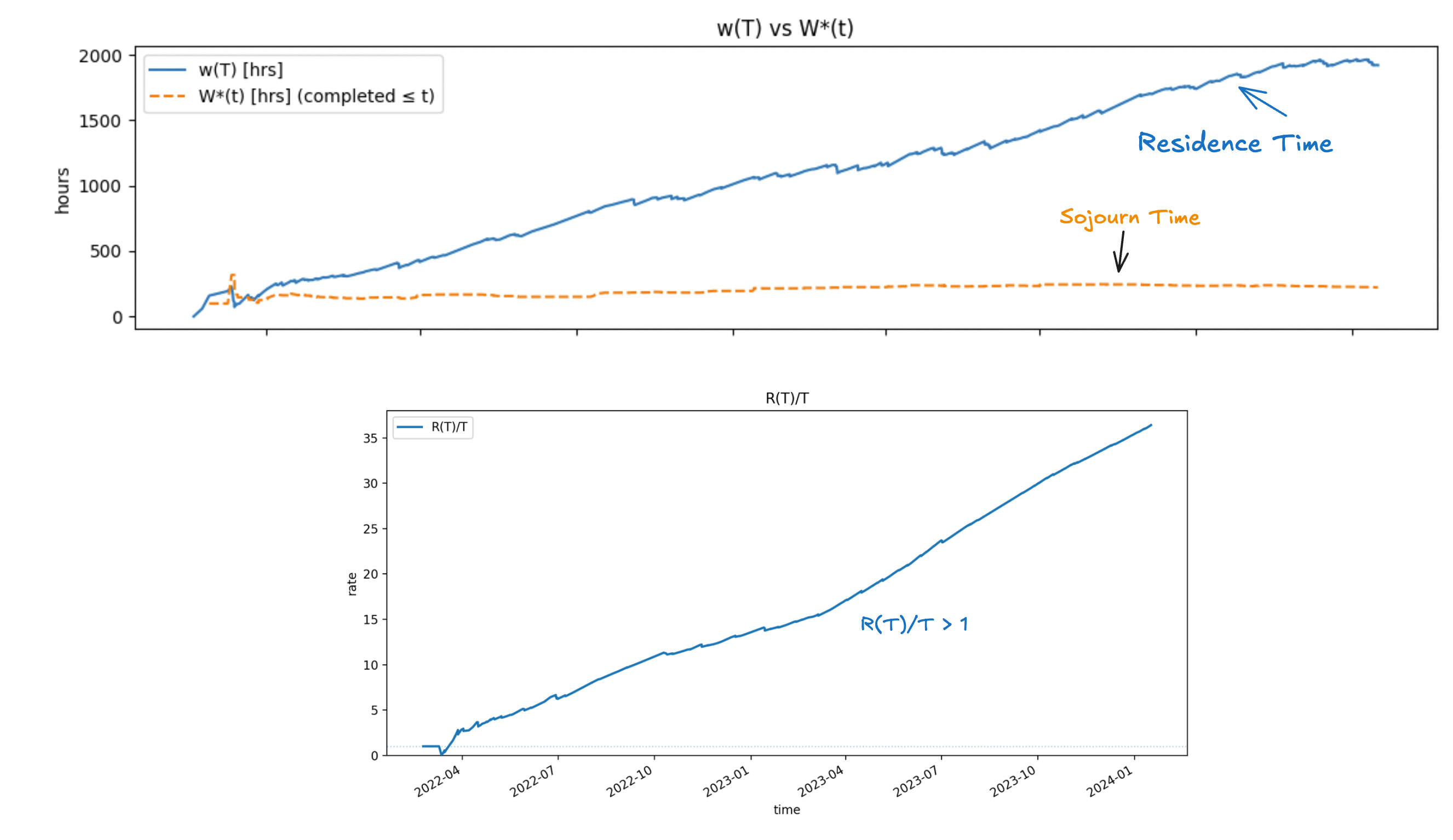
There are precise mathematical conditions for when this happens, and we can monitor for them in real-time. Let R(T) be the total age of the in-flight instances in the observation window.
Convergence is guaranteed if the total age of in-flight items grows sub-linearly with the length of your observation window, ie R(T)/T < 1 for all T.
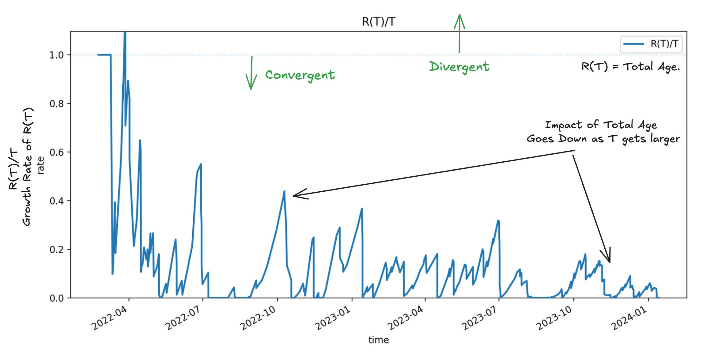
If total age grows linearly with the window length, the average residence time grows faster than the average sojourn time and two wont converge (see Fig 6). This typically means that you have long running instances that never complete so they keep adding residence time to the observation window, the longer you observe it and eventually total age swamps the sojourn times in total residence time.
So we have a few distinct possibilities each of which can be monitored for.
Convergent: Age contribution to the total shrinks over longer windows; the two averages move closer together. If they come together and stay there, we call the process stable.
Divergent: Total age dominates; the averages drift apart and sojourn time is no longer representative of true process time. Residence time still reflects true process time in this scenario.
Metastable: The process is convergent. The averages hover near each other but drift in and out of equality, even as the averages themselves change over time. Most real processes in a complex adaptive system live in this zone.
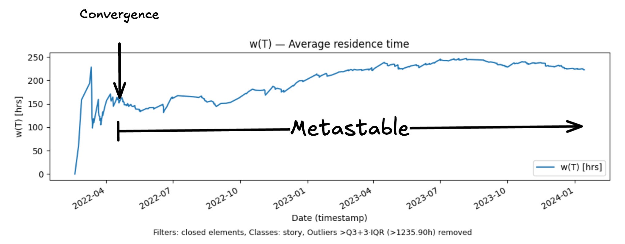
Metastable behavior represents a process operating in a dynamic equilibrium state, even though the average process time is changing. When average residence time and average sojourn times are equal we say that the process time measurement is coherent.
For more details on these concepts with precise mathematical definitions and detailed worked example please see Little’s Law in a Complex Adaptive System.
When process time is coherent, residence time is an accurate representation of sojourn time and both are accurate representations of process time. In particular, when process time is coherent, the process satisfies Little’s Law L=λW exactly.
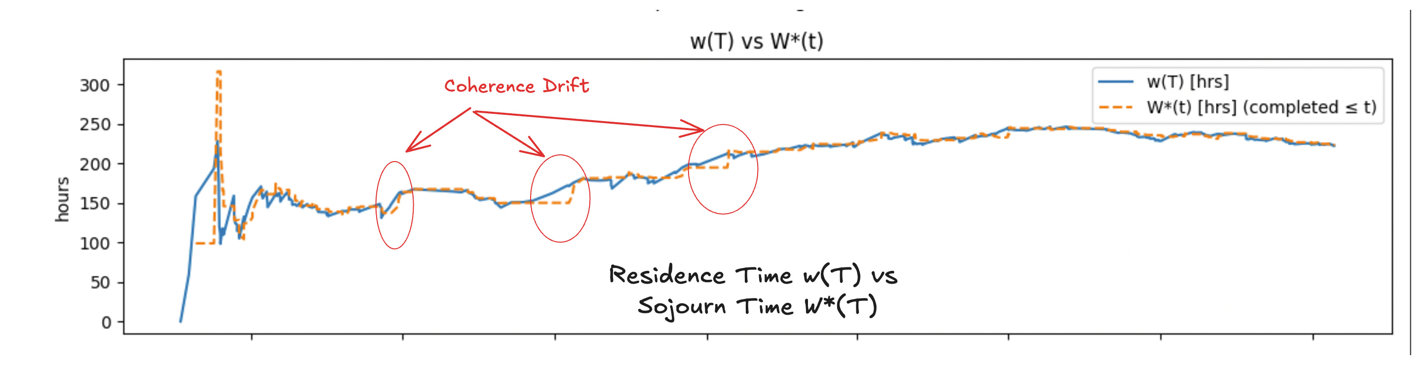
In metastable regimes, process time drifts in and out of coherence, but as Fig 8 shows, we can measure this precisely at any point in time.
If the difference between observed residence time and sojourn time at any point in time remains bounded, we also can place finite bounds on how well residence time serves as an estimate for sojourn time. If these bounds can be managed operationally through policies, this give us tools to manage the amount of epistemic uncertainty we tolerate for process time.
If it is impossible to bound this epistemic uncertainty through policy — say our process involves customers whose actions we cannot control — then we are operating in a fundamentally divergent process, and we should expect unbounded variation in process time and monitor and react to convergence or divergence as best as we can, rather than expecting we can control it.
This is a common situation in real-world complex adaptive systems.
Residence time as canonical process time
Regardless of whether the process is convergent or divergent, residence time remains the canonical measurement of process time for operational purposes. For any observation window [0,T] residence time w(T) is well defined, and it satisfies the finite version of Little’s Law:
and this holds whether the process is convergent, metastable or divergent.
Convergence or divergence concerns how this internally consistent measure relates to the externally reported sojourn time metric once you factor in epistemic uncertainty into the process. In this case, the difference between residence time and sojourn time represents the quantity we need to manage to.
How we mange it depends on the interpretation of process time. If we seek convergence, for example7, we can set tolerances for acceptable drift and growth rate for total age, and when they trigger investigate specific in-flight item(s) (and it is always in-flight items driving divergence) pulling the averages apart.
In our sales example deals could be aging for a variety of reasons:
Things are taking too long because of the nature of the deal or unexpected complications that arose in-flight,
They are stalled waiting for decisions, or
Because we have too many deals in flight and only a few are actually moving, the rest are waiting for attention.
A full causal analysis requires us to measure the other two parameters of Little’s Law and bring in additional domain context 8to help us understand why the process is diverging. We discussed this at a high level in The Causal Arrow in Little’s Law and show examples of the type of reasoning involved in Little’s Law in Complex Adaptive Systems.
If we seek divergence, then the strategies are usually flipped. For example if process time represents customer lifetime, then our strategies are going to conditioned on reducing customer churn and increasing process time.
In fig 9, we show an example of a process that we are managing for convergence, that has nevertheless slipped into a divergent state. We dont want to see this pattern if our goal is convergence, but the example does show that the growth rate of total age remains the lever that moves the process from convergence to divergence.
To Recap
For flow processes in a complex adaptive system, naïve elapsed time reports become polluted when the reporting window is much smaller than typical sojourn, and what is “typical” can’t be neatly quantified.
What you are seeing include significant distortions introduced by the measurement technique.
Instead, use sample path analysis to reveal the true, evolving, voice of the process:
Track residence time for both completed and in-flight items.
Watch whether unfinished age grows sub-linearly. If it does, average residence time ≈ average sojourn time, and you have a defensible, real-time answer to “how long does it take?” whether that is closing a deal, shipping a feature, or negotiating a contract.
If not, monitor whether residence times and sojourn times begin to diverge beyond your defined tolerance. When they do, investigate and intervene where possible. Where no interventions are possible, look for larger. systemic improvements that might be needed.
Now compared to the way process time is measured today we have
A sound metric, residence time, for “how long does it take?” that is not entangled with an observation window.
It works even with high variability and highly uncertain process times and is updated in real-time.
A live coherence check: are residence and sojourn averages agreeing within tolerance?
Action triggers: Any divergence beyond a set tolerance identifies that some action needs to be taken and the causal analysis using Little’s Law gives us a systematic way to track down potential sources of divergence. .
At each instant you have the best possible answer you can give for “how long does it take” and the tools to shape that answer to your needs.
The one thing to keep in mind here is that this entire analysis is entirely deterministic. We are in essence constructing a single, continuously updated sample of the process - a sample path, collecting cumulative process averages as we go along.
Any insights we get from this are specific to the process we study and for that process alone.
With complex adaptive systems this is the best we can do. What you are seeing when you observe over long enough periods, is the true voice of the specific process you are observing, free of measurement noise.
For most processes in complex adaptive systems there is no end date for how long you measure - the process itself is continuously evolving and the only thing you can compare the process with is its past self to understand how and where it is changing, and whether it needs to be nudged in a different direction.
This is what sample path analysis enables us to do - reveal the true, ongoing evolution of the voice of a flow process in a complex adaptive system.
But how long will it take?
Once you have a solid handle on answering “how long does it take”, we can turn to “how long will it take”. We’ll note that whether or not we can answer this depends on whether we can bound epistemic uncertainty.
In divergent processes, epistemic uncertainty grows without bound, so the only honest forecasts are distributions that acknowledge extreme tail risks. In convergent processes, epistemic uncertainty is bounded relative to the observation window, which opens the door to forecasting.
Residence time and convergence tests give us the foundation: they tell us when we are in a regime where forecasting is even meaningful.
Hint: Having a long run probability distribution over a convergent process and tools to detect when these probabilities change are key differentiators for forecasting driven by sample path analysis.
But that’s a subject for another post. We only promised to answer “how long does it take?” in this post!
In the next post in this series we will dive deeper to get more intuition about how residence time and sojourn time behave when the underlying processes are convergent or divergent. With lots of examples using real data!
Stay tuned or subscribe below if this is something are interested in learning more about.
For more details on how to calculate all these quantities precisely, and how the math works, see my post Little’s Law in a Complex Adaptive System.
That number also suffers from the same problem, but we’ll address that separately. Lets focus on process time first, because this is what drives that other number.
The voice of the process is a lovely term that I first read about in Donald Wheelers book: Understanding Variation. We use it here in the same sense as he does, but with the caveat that in a complex adaptive system we are usually not able to model the voice of the process using a stable distribution as is his baseline assumption. In fact, you may think of our usage of the term as how do you model the “voice of the process” when the process is inherently unpredictable.
The idea is that if we observe over long enough windows, whatever finite end-effects are there before the window will eventually become insignificant compared to the everything else in the window.
Conceptually this is an infinite window method, but in practice it may make sense to reset the starting point especially if very early segments of sample path history are no longer relevant to the current known operational state of the process. The key thing is that sample path analysis is history sensitive, a key requirement for analyzing process time in complex adaptive systems.
In operationa management settings, sojourn times are equivalent to what we would normally call Lead Time, Cycle Time, Flow Time etc. depending upon where process boundary was drawn. We use the more neutral term here because (1) this was the original term used in queueing theory where these problems were first studied (2) these other terms are context specific applications to specific processes in specific domains. Sample path theory and Little’s Law are domain agnostic.
Our lens for uncertainty is deterministic: we observe a single sample path that unfolds in time. We can observe up to the present, but we cannot see into the future. In this interpretation, end effects represent the uncertainty in what can be known, at a given time, about when ongoing process instances will complete.
Kim and Whitt tackle a related question from a more traditonal statistical perspective, treating end effects as contributors to the bias or variance of residence-time–based estimators for long-run averages of sojourn time. Their focus is on expectations of distributions across all sample paths in a stochastic process.
Almost all use cases we’ll find in use today seek convergence. But it is absolutely not the only way to operate these levers. Every one of these mechanisms can be used to tilt the process into divergent behavior when it means that divergence in the measurement leads to value being created, instead of cost or risks being accumulated. This is one of the major unrealized benefits of this machinery. Ultimately it’s about seeking convergence or divergence on time-value, not time itself.
We emphasize that sample path analysis is a domain agnostic measurement technique, and that’s all it is. It can accurately measure what is happening and detect proximate cause for a change in measurement using local mathematical cause-effect relationships. But it is not a standalone causal analysis tool. You cannot tell why something is happening in the domain or what actions you need to take to change the process behavior without bringing in specifics of the domain. But the triggers here will help focus what questions you should ask before you dip down into the domain level.